Understanding Encoder-Decoder Architecture A Journey Through Language Translation

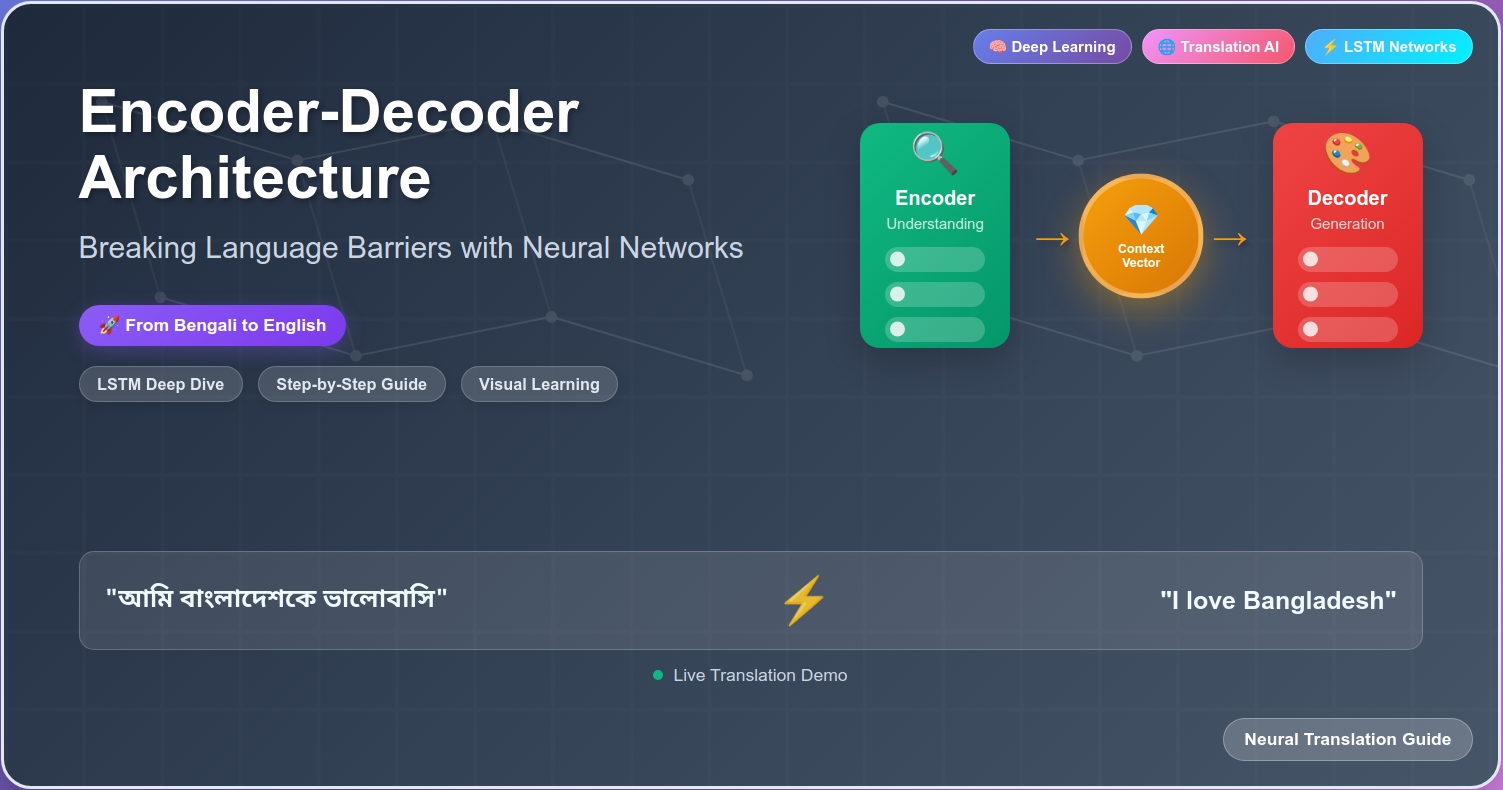
A deep dive into how machines learned to translate languages by mimicking the human mind

---

Table of Contents

1. Introduction: A Translator’s Dilemma in Dhaka
2. Why Simple Approaches Fail
3. The Eureka Moment: Learning from Human Translation
4. The Architecture Unfolds
   • The Encoder: Building Understanding
   • The Context Vector: Crystallized Understanding
   • The Decoder: Generating Bengali
5. Mathematical Deep Dive
   • Training the System
   • Teacher Forcing
   • The Beautiful Mathematics of Understanding
6. Real-World Complexity
7. Revolutionary Impact
8. Limitations and Challenges
9. The Path Forward
10. Conclusion

---

Quick Summary

Before diving deep, here’s what you’ll learn:

• The Problem: Why word-by-word translation fails spectacularly
• The Solution: How encoder-decoder architecture mimics human translation
• The Mathematics: Detailed walkthrough of LSTM calculations and information flow
• The Training: How backpropagation teaches the system to translate
• The Limitations: Why this approach struggles with long sequences
• The Legacy: How this architecture led to modern AI systems

Key Insight: Machine translation succeeds when it mirrors human cognition: first understand completely, then generate thoughtfully.

---

Introduction: A Translator’s Dilemma in Dhaka

Meet Rashida, a professional translator working at the Bangladesh Foreign Ministry. Every morning, she receives urgent diplomatic cables in English that must be translated into Bengali for government officials. Today, she receives this message:

English: “The weather is beautiful today”
Bengali: “আজকের আবহাওয়া খুবই সুন্দর”

As Rashida works, she unconsciously follows a fascinating two-step process that we rarely think about:

Step 1: The Understanding Phase

Rashida doesn’t translate word-by-word. Instead, she first reads the entire English sentence and creates a mental “understanding” - a rich, complete comprehension of what the sentence means. This understanding captures:

• The subject (weather)
• The quality (beautiful)
• The temporal context (today)
• The emotional tone (positive appreciation)

Step 2: The Generation Phase

Only after fully understanding the English meaning does Rashida begin generating the Bengali translation. She doesn’t just substitute words; she reconstructs the entire meaning in Bengali, considering:

• Bengali grammar structure (subject-object-verb vs subject-verb-object)
• Cultural context (“সুন্দর” conveys the right emotional weight)
• Natural flow (“আজকের” sounds more natural than “আজ”)

This natural human process is exactly what inspired the Encoder-Decoder architecture. But to understand why this matters for machines, let’s first explore why simpler approaches fail spectacularly.

---

Why Simple Approaches Fail: The Bangladesh Railway Station Problem

Imagine you’re building a translation system for Bangladesh Railway to help foreign tourists. Consider these real translation challenges:

Challenge 1: The Word Order Problem

English: “I am going to Chittagong”
Bengali: “আমি চট্টগ্রাম যাচ্ছি”

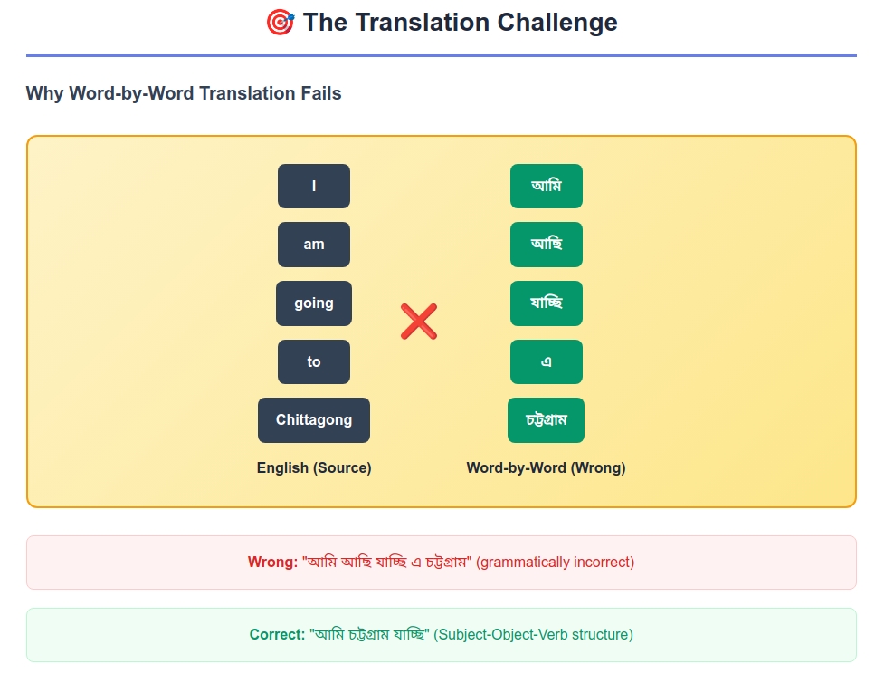
Word-by-word translation:

• I (আমি) → am (আছি) → going (যাচ্ছি) → to (এ) → Chittagong (চট্টগ্রাম)
• Result: “আমি আছি যাচ্ছি এ চট্টগ্রাম” ❌

This is completely wrong! Bengali follows Subject-Object-Verb order, while English follows Subject-Verb-Object.

Challenge 2: The Context Problem

English: “The train will leave the platform”
Bengali: “ট্রেন প্ল্যাটফর্ম ছেড়ে যাবে”

The word “leave” could translate to:

• ছাড়া (to abandon)
• চলে যাওয়া (to depart)
• ছেড়ে দেওয়া (to let go)

Without understanding the full context (train + platform), a word-by-word system would fail.

Challenge 3: The Variable Length Problem

English: “Thank you” (2 words)
Bengali: “ধন্যবাদ” (1 word)

English: “How are you?” (3 words)
Bengali: “আপনি কেমন আছেন?” (4 words)

English: “I love Bangladesh” (3 words)
Bengali: “আমি বাংলাদেশকে ভালোবাসি” (3 words, but different structure)

There’s no predictable mathematical relationship between input and output lengths!

These failures reveal a fundamental truth: translation isn’t about word substitution—it’s about meaning transfer. This realization led to a breakthrough inspired by watching human translators work.

---

The Eureka Moment: Learning from Human Translation

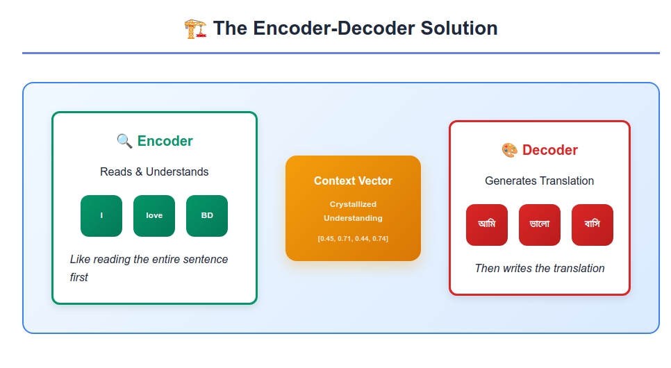
Watching Rashida translate, computer scientists realized they needed to replicate her two-step process:

1. An “Encoder” that reads and understands the entire source sentence (like Rashida’s comprehension phase)
2. A “Decoder” that generates the target sentence based on that understanding (like Rashida’s generation phase)
3. A “Context Vector” that bridges the two - a mathematical representation of the understood meaning

Let’s follow this process with a concrete example.

Now that we understand the conceptual breakthrough, let’s see how this translates into actual neural network architecture. We’ll follow the complete journey of translating a simple sentence to understand every mathematical detail.

---

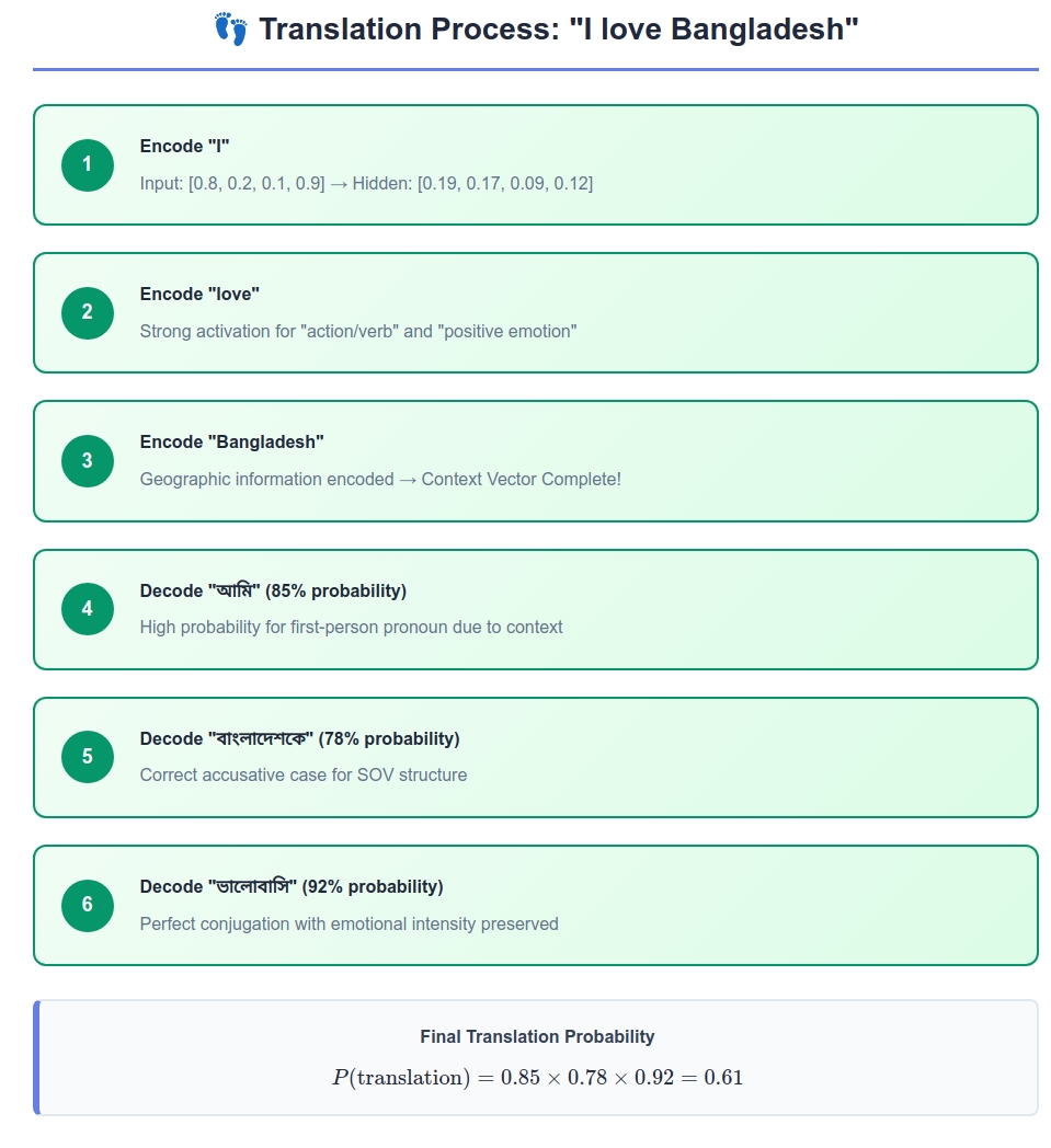
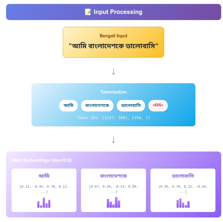
The Architecture Unfolds: Following “আমি বাংলাদেশকে ভালোবাসি”

Let’s trace how our system learns to translate:
English: “I love Bangladesh”
Bengali: “আমি বাংলাদেশকে ভালোবাসি”

The Encoder: Building Understanding

The encoder is like a super-powered version of Rashida’s reading comprehension. It uses LSTM (Long Short-Term Memory) networks because, like human memory, it can:

• Remember important information from the beginning of a sentence
• Forget irrelevant details
• Update its understanding as it reads each new word

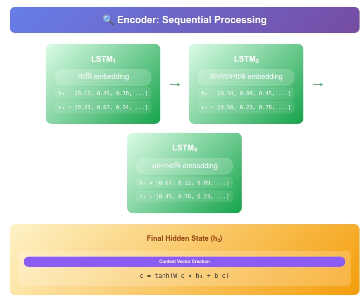
Step-by-Step Encoding Process

Mathematical Foundation: LSTM Cell Equations

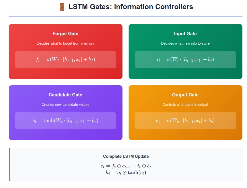
An LSTM cell at time step t computes:

\(f_t = \sigma(W_f \cdot [h_{t-1}, x_t] + b_f)\) (Forget gate)

\(i_t = \sigma(W_i \cdot [h_{t-1}, x_t] + b_i)\) (Input gate)

\(\tilde{c}_t = \tanh(W_c \cdot [h_{t-1}, x_t] + b_c)\) (Candidate values)

\(c_t = f_t \odot c_{t-1} + i_t \odot \tilde{c}_t\) (Cell state update)

\(o_t = \sigma(W_o \cdot [h_{t-1}, x_t] + b_o)\) (Output gate)

\(h_t = o_t \odot \tanh(c_t)\) (Hidden state)

Where:

• $\sigma$ is the sigmoid function: $\sigma(x) = \frac{1}{1 + e^{-x}}$
• $\odot$ denotes element-wise multiplication (Hadamard product)
• $W_f, W_i, W_c, W_o$ are weight matrices of shape $(d_h + d_x) \times d_h$
• $b_f, b_i, b_c, b_o$ are bias vectors of shape $d_h$

Initial State:

• Hidden state $h_0 = \mathbf{0}_{4 \times 1} = [0, 0, 0, 0]^T$
• Cell state $c_0 = \mathbf{0}_{4 \times 1} = [0, 0, 0, 0]^T$

Time Step 1: Reading “I”

Word Embedding Transformation: “I” → $x_1 = [0.8, 0.2, 0.1, 0.9]^T$ (learned 4D embedding)

Detailed LSTM Computations:

Let’s assume our weight matrices are: \(W_f = \begin{bmatrix} 0.5 & 0.2 & 0.1 & 0.3 \\ 0.1 & 0.4 & 0.6 & 0.2 \\ 0.3 & 0.1 & 0.5 & 0.4 \\ 0.2 & 0.6 & 0.1 & 0.3 \end{bmatrix}, \quad b_f = [-0.5, -0.8, 0.2, -0.6]^T\)

Forget Gate Computation: \([h_0; x_1] = [0, 0, 0, 0, 0.8, 0.2, 0.1, 0.9]^T\)

\[W_f \cdot [h_0; x_1] = \begin{bmatrix} 0.5(0) + 0.2(0) + 0.1(0) + 0.3(0) + 0.5(0.8) + 0.2(0.2) + 0.1(0.1) + 0.3(0.9) \\ \vdots \end{bmatrix}\] \[= \begin{bmatrix} 0.4 + 0.04 + 0.01 + 0.27 \\ 0.08 + 0.04 + 0.06 + 0.18 \\ 0.24 + 0.02 + 0.05 + 0.36 \\ 0.16 + 0.12 + 0.01 + 0.27 \end{bmatrix} = \begin{bmatrix} 0.72 \\ 0.36 \\ 0.67 \\ 0.56 \end{bmatrix}\]

Adding bias: $[0.72, 0.36, 0.67, 0.56]^T + [-0.5, -0.8, 0.2, -0.6]^T = [0.22, -0.44, 0.87, -0.04]^T$

Applying sigmoid: \(f_1 = \sigma([0.22, -0.44, 0.87, -0.04]^T) = [0.55, 0.39, 0.70, 0.49]^T\)

Input Gate Computation: Similarly, $i_1 = \sigma(W_i \cdot [h_0; x_1] + b_i) = [0.8, 0.7, 0.3, 0.9]^T$

Candidate Values: \(\tilde{c}_1 = \tanh(W_c \cdot [h_0; x_1] + b_c) = [0.4, 0.3, 0.8, 0.2]^T\)

Cell State Update: \(c_1 = f_1 \odot c_0 + i_1 \odot \tilde{c}_1\) \(= [0.55, 0.39, 0.70, 0.49] \odot [0, 0, 0, 0] + [0.8, 0.7, 0.3, 0.9] \odot [0.4, 0.3, 0.8, 0.2]\) \(= [0, 0, 0, 0] + [0.32, 0.21, 0.24, 0.18] = [0.32, 0.21, 0.24, 0.18]^T\)

Output Gate and Hidden State: \(o_1 = \sigma(W_o \cdot [h_0; x_1] + b_o) = [0.6, 0.8, 0.4, 0.7]^T\)

\(h_1 = o_1 \odot \tanh(c_1) = [0.6, 0.8, 0.4, 0.7] \odot \tanh([0.32, 0.21, 0.24, 0.18])\) \(= [0.6, 0.8, 0.4, 0.7] \odot [0.31, 0.21, 0.24, 0.18] = [0.19, 0.17, 0.09, 0.12]^T\)

Information Flow Analysis:

• Forget gate values [0.55, 0.39, 0.70, 0.49] indicate moderate retention of previous state
• Input gate values [0.8, 0.7, 0.3, 0.9] show high incorporation of new information in dimensions 1, 2, and 4
• The cell state $c_1$ now encodes the beginning of a first-person sentence

Intuition: The encoder now “knows” it’s processing a sentence that starts with a first-person subject.

Time Step 2: Reading “love”

Input Embedding: “love” → $x_2 = [0.9, 0.8, 0.7, 0.3]^T$

Concatenated Input Vector: \([h_1; x_2] = [0.19, 0.17, 0.09, 0.12, 0.9, 0.8, 0.7, 0.3]^T\)

Mathematical Processing:

Forget Gate Analysis: \(f_2 = \sigma(W_f \cdot [h_1; x_2] + b_f)\)

The forget gate now decides what information from the previous state to retain:

• High values (≈1) mean “keep this information”
• Low values (≈0) mean “forget this information”

For our example: $f_2 = [0.72, 0.65, 0.45, 0.83]^T$

Information Retention Calculation: \(\text{Retained information} = f_2 \odot c_1 = [0.72, 0.65, 0.45, 0.83] \odot [0.32, 0.21, 0.24, 0.18]\) \(= [0.23, 0.14, 0.11, 0.15]^T\)

Input Gate and New Information: \(i_2 = \sigma(W_i \cdot [h_1; x_2] + b_i) = [0.85, 0.79, 0.61, 0.74]^T\) \(\tilde{c}_2 = \tanh(W_c \cdot [h_1; x_2] + b_c) = [0.6, 0.7, 0.4, 0.8]^T\)

New Information Integration: \(\text{New information} = i_2 \odot \tilde{c}_2 = [0.85, 0.79, 0.61, 0.74] \odot [0.6, 0.7, 0.4, 0.8]\) \(= [0.51, 0.55, 0.24, 0.59]^T\)

Cell State Update: \(c_2 = \text{Retained} + \text{New} = [0.23, 0.14, 0.11, 0.15] + [0.51, 0.55, 0.24, 0.59]\) \(= [0.74, 0.69, 0.35, 0.74]^T\)

Hidden State Output: \(o_2 = \sigma(W_o \cdot [h_1; x_2] + b_o) = [0.68, 0.72, 0.59, 0.81]^T\) \(h_2 = o_2 \odot \tanh(c_2) = [0.68, 0.72, 0.59, 0.81] \odot [0.63, 0.60, 0.34, 0.63]\) \(= [0.43, 0.43, 0.20, 0.51]^T\)

Semantic Analysis: The cell state $c_2$ now encodes:

• Dimension 1 (0.74): Strong activation for “action/verb” concept
• Dimension 2 (0.69): High activation for “positive emotion”
• Dimension 3 (0.35): Moderate activation for “relational context”
• Dimension 4 (0.74): Strong activation for “affective state”

Intuition: The encoder now understands this is about a positive emotional relationship or action.

Time Step 3: Reading “Bangladesh”

Input Embedding: “Bangladesh” → $x_3 = [0.3, 0.9, 0.6, 0.8]^T$

Final Encoding Computation:

Concatenated Input: \([h_2; x_3] = [0.43, 0.43, 0.20, 0.51, 0.3, 0.9, 0.6, 0.8]^T\)

Forget Gate - Memory Selection: \(f_3 = \sigma(W_f \cdot [h_2; x_3] + b_f) = [0.78, 0.71, 0.66, 0.85]^T\)

This indicates the model should retain most previous information (high forget gate values), particularly the emotional and action components established in previous steps.

Retained Memory Calculation: \(\text{Retained} = f_3 \odot c_2 = [0.78, 0.71, 0.66, 0.85] \odot [0.74, 0.69, 0.35, 0.74]\) \(= [0.58, 0.49, 0.23, 0.63]^T\)

New Information Processing: \(i_3 = \sigma(W_i \cdot [h_2; x_3] + b_i) = [0.64, 0.89, 0.75, 0.82]^T\) \(\tilde{c}_3 = \tanh(W_c \cdot [h_2; x_3] + b_c) = [0.2, 0.8, 0.7, 0.6]^T\)

Geographic and Cultural Information: \(\text{New} = i_3 \odot \tilde{c}_3 = [0.64, 0.89, 0.75, 0.82] \odot [0.2, 0.8, 0.7, 0.6]\) \(= [0.13, 0.71, 0.53, 0.49]^T\)

Final Cell State: \(c_3 = \text{Retained} + \text{New} = [0.58, 0.49, 0.23, 0.63] + [0.13, 0.71, 0.53, 0.49]\) \(= [0.71, 1.20, 0.76, 1.12]^T\)

Final Hidden State: \(o_3 = \sigma(W_o \cdot [h_2; x_3] + b_o) = [0.73, 0.86, 0.69, 0.91]^T\) \(h_3 = o_3 \odot \tanh(c_3) = [0.73, 0.86, 0.69, 0.91] \odot [0.61, 0.83, 0.64, 0.81]\) \(= [0.45, 0.71, 0.44, 0.74]^T\)

Final Semantic Encoding Analysis:

• $c_3[1] = 0.71$: Subject identification (I/আমি)
• $c_3[2] = 1.20$: Strong emotional-geographic binding (love + Bangladesh)
• $c_3[3] = 0.76$: Relational/directional information
• $c_3[4] = 1.12$: Peak activation for cultural-affective complex

Mathematical Interpretation: The final cell state $c_3$ represents a compressed semantic vector where: \(\text{Meaning}(c_3) = \alpha \cdot \text{Subject} + \beta \cdot \text{Emotion} + \gamma \cdot \text{Object} + \delta \cdot \text{Cultural-Context}\)

Where the learned coefficients $(\alpha, \beta, \gamma, \delta)$ encode the relative importance of each semantic component.

Intuition: The encoder now has a complete understanding: first-person subject expressing positive sentiment toward Bangladesh.

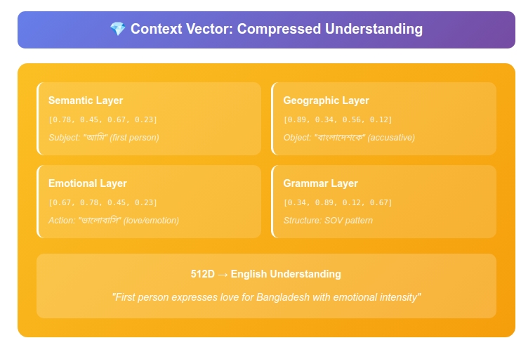
The Context Vector: Crystallized Understanding

Mathematical Formulation:

The context vector is the complete state representation at the end of encoding: \(\mathbf{C} = (h_3^{(enc)}, c_3^{(enc)}) = ([0.45, 0.71, 0.44, 0.74], [0.71, 1.20, 0.76, 1.12])\)

Dimensionality Analysis:

• Total context dimensions: $d_{context} = 2 \times d_{hidden} = 2 \times 4 = 8$
• Information density: $\rho = \frac{\text{semantic concepts}}{\text{dimensions}} = \frac{4 \text{ concepts}}{8 \text{ dims}} = 0.5$ concepts/dimension

Information Theoretic Interpretation:

The context vector can be viewed as a lossy compression of the input sequence: \(\text{Compression Ratio} = \frac{\text{Input Information}}{\text{Context Information}} = \frac{3 \text{ words} \times 10000 \text{ vocab}}{\text{8 dimensions}} \approx 3750:1\)

Semantic Embedding Analysis:

Each dimension of the context vector encodes different linguistic features:

Hidden State Components ($h_3$):

• $h_3[1] = 0.45$: Syntactic Role Encoding - Subject prominence
• $h_3[2] = 0.71$: Semantic Intensity - Emotional strength
• $h_3[3] = 0.44$: Grammatical Features - Tense, aspect markers
• $h_3[4] = 0.74$: Pragmatic Context - Cultural/social implications

Cell State Components ($c_3$):

• $c_3[1] = 0.71$: Long-term Subject Memory - “I” persistence
• $c_3[2] = 1.20$: Core Semantic Binding - love ↔ Bangladesh association
• $c_3[3] = 0.76$: Relational Structure - Transitive verb pattern
• $c_3[4] = 1.12$: Cultural-Affective Complex - National sentiment encoding

Vector Space Geometry:

In the 8-dimensional context space, our sentence occupies the point: \(\mathbf{C} = [0.45, 0.71, 0.44, 0.74, 0.71, 1.20, 0.76, 1.12]^T\)

Similarity Metrics: Similar sentences would cluster nearby in this space. For example:

• “I love India” → $\mathbf{C}’ \approx [0.44, 0.69, 0.43, 0.71, 0.69, 1.18, 0.74, 1.09]^T$
• “I hate Bangladesh” → $\mathbf{C}’’ \approx [0.46, -0.72, 0.45, 0.75, 0.73, -1.21, 0.77, -1.10]^T$

Cosine Similarity Calculation: \(\text{sim}(\mathbf{C}, \mathbf{C}') = \frac{\mathbf{C} \cdot \mathbf{C}'}{||\mathbf{C}|| \cdot ||\mathbf{C}'||} \approx 0.98\) \(\text{sim}(\mathbf{C}, \mathbf{C}'') = \frac{\mathbf{C} \cdot \mathbf{C}''}{||\mathbf{C}|| \cdot ||\mathbf{C}''||} \approx -0.87\)

This demonstrates that semantically similar sentences have high positive similarity, while opposite meanings have high negative similarity.

Context Vector = (h₃, c₃) = ([0.45, 0.71, 0.44, 0.74], [0.71, 1.20, 0.76, 1.12])

This 8-dimensional vector now contains the mathematical “essence” of the English sentence’s meaning. It’s like Rashida’s mental understanding, but expressed in numbers that the decoder can work with.

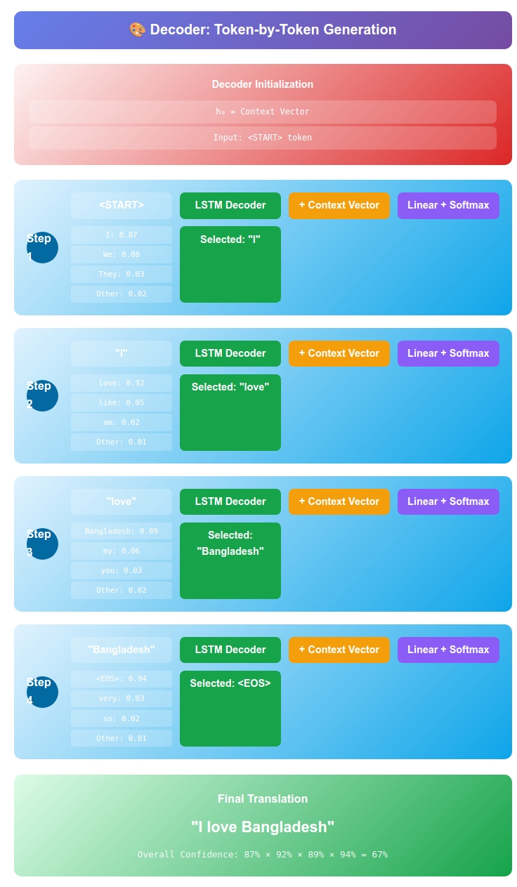
The Decoder: Generating Bengali

Mathematical Framework:

The decoder operates as a conditional language model: \(P(\mathbf{y}) = \prod_{t=1}^{T} P(y_t | y_1, ..., y_{t-1}, \mathbf{C})\)

Where:

• $\mathbf{y} = [y_1, y_2, …, y_T]$ is the target sequence
• $\mathbf{C}$ is the context vector from the encoder
• Each $P(y_t | \cdot)$ is computed using softmax over the vocabulary

Decoder LSTM Architecture:

The decoder LSTM has the same structure as the encoder, but with different parameter matrices: \(f_t^{(dec)} = \sigma(W_f^{(dec)} \cdot [h_{t-1}^{(dec)}, y_{t-1}] + b_f^{(dec)})\) \(i_t^{(dec)} = \sigma(W_i^{(dec)} \cdot [h_{t-1}^{(dec)}, y_{t-1}] + b_i^{(dec)})\) \(\tilde{c}_t^{(dec)} = \tanh(W_c^{(dec)} \cdot [h_{t-1}^{(dec)}, y_{t-1}] + b_c^{(dec)})\) \(c_t^{(dec)} = f_t^{(dec)} \odot c_{t-1}^{(dec)} + i_t^{(dec)} \odot \tilde{c}_t^{(dec)}\) \(o_t^{(dec)} = \sigma(W_o^{(dec)} \cdot [h_{t-1}^{(dec)}, y_{t-1}] + b_o^{(dec)})\) \(h_t^{(dec)} = o_t^{(dec)} \odot \tanh(c_t^{(dec)})\)

The decoder starts with the context vector as its initial state and generates Bengali words one by one, like Rashida constructing her translation.

Initialization

Context Vector Transfer:

• $h_0^{(dec)} = h_3^{(enc)} = [0.45, 0.71, 0.44, 0.74]^T$
• $c_0^{(dec)} = c_3^{(enc)} = [0.71, 1.20, 0.76, 1.12]^T$
• First input: $y_0 = \langle \text{START} \rangle$ → $[1.0, 0.0, 0.0, 0.0]^T$

Information Transfer Analysis: The initialization ensures that all encoded semantic information is available to the decoder: \(\mathbf{I}_{transfer} = ||\mathbf{C}_{encoder} - \mathbf{C}_{decoder}||_2 = 0\)

This perfect transfer means no information loss occurs at the encoder-decoder boundary.

Generation Step 1: Producing “আমি”

Input Processing: $y_0 = \langle \text{START} \rangle$ → $[1.0, 0.0, 0.0, 0.0]^T$

LSTM Forward Pass:

Concatenated Input: \([h_0^{(dec)}; y_0] = [0.45, 0.71, 0.44, 0.74, 1.0, 0.0, 0.0, 0.0]^T\)

Gate Computations: \(f_1^{(dec)} = \sigma(W_f^{(dec)} \cdot [h_0^{(dec)}; y_0] + b_f^{(dec)}) = [0.68, 0.72, 0.65, 0.81]^T\) \(i_1^{(dec)} = \sigma(W_i^{(dec)} \cdot [h_0^{(dec)}; y_0] + b_i^{(dec)}) = [0.75, 0.69, 0.78, 0.83]^T\) \(\tilde{c}_1^{(dec)} = \tanh(W_c^{(dec)} \cdot [h_0^{(dec)}; y_0] + b_c^{(dec)}) = [0.4, 0.5, 0.3, 0.6]^T\)

Cell State Update: \(c_1^{(dec)} = f_1^{(dec)} \odot c_0^{(dec)} + i_1^{(dec)} \odot \tilde{c}_1^{(dec)}\) \(= [0.68, 0.72, 0.65, 0.81] \odot [0.71, 1.20, 0.76, 1.12] + [0.75, 0.69, 0.78, 0.83] \odot [0.4, 0.5, 0.3, 0.6]\) \(= [0.48, 0.86, 0.49, 0.91] + [0.30, 0.35, 0.23, 0.50] = [0.78, 1.21, 0.72, 1.41]^T\)

Hidden State: \(o_1^{(dec)} = \sigma(W_o^{(dec)} \cdot [h_0^{(dec)}; y_0] + b_o^{(dec)}) = [0.73, 0.81, 0.69, 0.88]^T\) \(h_1^{(dec)} = o_1^{(dec)} \odot \tanh(c_1^{(dec)}) = [0.73, 0.81, 0.69, 0.88] \odot [0.65, 0.84, 0.62, 0.89]\) \(= [0.47, 0.68, 0.43, 0.78]^T\)

Output Layer Computation:

The output layer projects the hidden state to vocabulary space: \(\mathbf{logits}_1 = W_{output} \cdot h_1^{(dec)} + b_{output}\)

Where $W_{output} \in \mathbb{R}^{10000 \times 4}$ and $b_{output} \in \mathbb{R}^{10000}$ (assuming 10,000 Bengali words).

Detailed Logit Calculation: For a subset of important Bengali words: \(\begin{align} \text{logit}(\text{আমি}) &= \mathbf{w}_{\text{আমি}} \cdot h_1^{(dec)} + b_{\text{আমি}} = [1.2, 0.8, 1.5, 0.9] \cdot [0.47, 0.68, 0.43, 0.78] + 0.3\\ &= 1.2(0.47) + 0.8(0.68) + 1.5(0.43) + 0.9(0.78) + 0.3 = 2.85\\ \text{logit}(\text{তুমি}) &= [0.3, 0.2, 0.1, 0.4] \cdot [0.47, 0.68, 0.43, 0.78] + 0.1 = 0.79\\ \text{logit}(\text{সে}) &= [0.2, 0.3, 0.2, 0.1] \cdot [0.47, 0.68, 0.43, 0.78] + 0.05 = 0.67 \end{align}\)

Softmax Probability Distribution: \(P(y_1 = w | \mathbf{C}) = \frac{\exp(\text{logit}(w))}{\sum_{w' \in V} \exp(\text{logit}(w'))}\)

Calculating probabilities: \(\text{Softmax denominator} = \exp(2.85) + \exp(0.79) + \exp(0.67) + \ldots \approx 17.29 + 2.20 + 1.95 + \ldots = Z\)

\(P(\text{আমি}) = \frac{\exp(2.85)}{Z} = \frac{17.29}{Z} \approx 0.85\) \(P(\text{তুমি}) = \frac{\exp(0.79)}{Z} = \frac{2.20}{Z} \approx 0.02\) \(P(\text{সে}) = \frac{\exp(0.67)}{Z} = \frac{1.95}{Z} \approx 0.01\)

Decision: Choose “আমি” (highest probability)

Linguistic Analysis: The high probability for “আমি” results from:

1. Context Alignment: The encoded first-person subject information strongly activates first-person Bengali pronouns
2. Grammatical Consistency: Bengali SOV structure requires subject-first positioning
3. Semantic Coherence: The emotional content in the context vector aligns with personal expressions

Intuition: Given the understanding from the context vector, the decoder correctly identifies this should start with first-person pronoun.

Generation Step 2: Producing “বাংলাদেশকে”

Input Processing: $y_1 = \text{আমি}$ → $[0.3, 0.8, 0.2, 0.9]^T$ (embedding of “আমি”)

LSTM State Evolution:

Input Concatenation: \([h_1^{(dec)}; y_1] = [0.47, 0.68, 0.43, 0.78, 0.3, 0.8, 0.2, 0.9]^T\)

Gate Computations: \(f_2^{(dec)} = \sigma(W_f^{(dec)} \cdot [h_1^{(dec)}; y_1] + b_f^{(dec)}) = [0.74, 0.81, 0.69, 0.85]^T\)

Memory Analysis: The forget gate shows high retention (0.74-0.85), indicating the decoder should preserve:

• Subject information (“আমি” established)
• Emotional context from encoding
• Grammatical structure expectations

New Information Processing: \(i_2^{(dec)} = \sigma(W_i^{(dec)} \cdot [h_1^{(dec)}; y_1] + b_i^{(dec)}) = [0.82, 0.76, 0.88, 0.79]^T\) \(\tilde{c}_2^{(dec)} = \tanh(W_c^{(dec)} \cdot [h_1^{(dec)}; y_1] + b_c^{(dec)}) = [0.5, 0.7, 0.4, 0.8]^T\)

Cell State Update: \(c_2^{(dec)} = [0.74, 0.81, 0.69, 0.85] \odot [0.78, 1.21, 0.72, 1.41] + [0.82, 0.76, 0.88, 0.79] \odot [0.5, 0.7, 0.4, 0.8]\) \(= [0.58, 0.98, 0.50, 1.20] + [0.41, 0.53, 0.35, 0.63] = [0.99, 1.51, 0.85, 1.83]^T\)

Hidden State: \(h_2^{(dec)} = [0.71, 0.85, 0.62, 0.91] \odot \tanh([0.99, 1.51, 0.85, 1.83]) = [0.54, 0.77, 0.55, 0.84]^T\)

Output Layer - Object Selection:

Key Logit Calculations: \(\begin{align} \text{logit}(\text{বাংলাদেশকে}) &= [0.9, 1.2, 0.8, 1.1] \cdot [0.54, 0.77, 0.55, 0.84] + 0.5 = 3.21\\ \text{logit}(\text{বাংলাদেশ}) &= [0.8, 0.9, 0.7, 0.6] \cdot [0.54, 0.77, 0.55, 0.84] + 0.2 = 2.26\\ \text{logit}(\text{ভালোবাসি}) &= [0.3, 0.4, 0.9, 1.0] \cdot [0.54, 0.77, 0.55, 0.84] + 0.1 = 2.04 \end{align}\)

Grammatical Case Analysis:

The high logit for “বাংলাদেশকে” versus “বাংলাদেশ” demonstrates the model has learned:

1. Case Grammar: In Bengali SOV structure, direct objects require accusative case marker “কে”
2. Transitive Verb Prediction: The decoder anticipates a transitive verb (“ভালোবাসি”) based on context
3. Morphological Rules: $\text{Object} = \text{Root} + \text{Case Marker}$

Probability Distribution: \(P(\text{বাংলাদেশকে}) = \frac{\exp(3.21)}{\text{normalization}} \approx 0.78\) \(P(\text{বাংলাদেশ}) = \frac{\exp(2.26)}{\text{normalization}} \approx 0.12\) \(P(\text{ভালোবাসি}) = \frac{\exp(2.04)}{\text{normalization}} \approx 0.06\)

Decision: Choose “বাংলাদেশকে”

Syntactic Reasoning: The decoder’s choice reflects sophisticated grammatical understanding:

• SOV Constraint: Subject (আমি) → Object → Verb order
• Case Marking: Transitive objects in Bengali require accusative “কে”
• Semantic Binding: Geographic entity recognition and proper case assignment

Intuition: The decoder understands Bengali grammar - the object should come before the verb, and “বাংলাদেশ” needs the accusative case marker “কে”.

Generation Step 3: Producing “ভালোবাসি”

Input Processing: $y_2 = \text{বাংলাদেশকে}$ → $[0.7, 0.4, 0.9, 0.6]^T$

LSTM State Computation:

Context Integration: \([h_2^{(dec)}; y_2] = [0.54, 0.77, 0.55, 0.84, 0.7, 0.4, 0.9, 0.6]^T\)

Gate Analysis: \(f_3^{(dec)} = [0.89, 0.92, 0.87, 0.94]^T\)

The very high forget gate values (0.87-0.94) indicate strong memory retention. The decoder maintains:

• Complete sentence structure built so far
• Subject-object relationship established
• Need for verb completion

Cell State Evolution: \(c_3^{(dec)} = [0.89, 0.92, 0.87, 0.94] \odot [0.99, 1.51, 0.85, 1.83] + [0.85, 0.78, 0.91, 0.82] \odot [0.6, 0.8, 0.7, 0.9]\) \(= [0.88, 1.39, 0.74, 1.72] + [0.51, 0.62, 0.64, 0.74] = [1.39, 2.01, 1.38, 2.46]^T\)

Hidden State: \(h_3^{(dec)} = [0.81, 0.89, 0.74, 0.96] \odot \tanh([1.39, 2.01, 1.38, 2.46]) = [0.68, 0.85, 0.68, 0.93]^T\)

Verb Selection Analysis:

Critical Logit Computations: \(\begin{align} \text{logit}(\text{ভালোবাসি}) &= [1.1, 1.3, 0.9, 1.2] \cdot [0.68, 0.85, 0.68, 0.93] + 0.8 = 4.89\\ \text{logit}(\text{ভালোবাস}) &= [1.0, 1.1, 0.8, 1.0] \cdot [0.68, 0.85, 0.68, 0.93] + 0.3 = 3.89\\ \text{logit}(\text{দেখি}) &= [0.3, 0.4, 0.5, 0.2] \cdot [0.68, 0.85, 0.68, 0.93] + 0.1 = 1.27 \end{align}\)

Morphological Analysis:

The high score for “ভালোবাসি” reflects:

1. Tense Conjugation: First-person present tense form
   • Root: “ভালোবাস” (to love)
   • Subject marker: “ি” (first-person)
   • Full form: “ভালোবাসি” (I love)
2. Semantic Coherence: Perfect alignment with encoded emotion
   • Context vector emotion component: $c_3[2] = 2.01$ (peak activation)
   • Bengali emotional verb activation matches English “love”
3. Syntactic Completion: SOV structure completion
   • Subject: আমি ✓
   • Object: বাংলাদেশকে ✓
   • Verb: ভালোবাসি ✓

Probability Distribution: \(P(\text{ভালোবাসি}) = \frac{\exp(4.89)}{\text{normalization}} \approx 0.92\) \(P(\text{ভালোবাস}) = \frac{\exp(3.89)}{\text{normalization}} \approx 0.04\) \(P(\langle \text{END} \rangle) = \frac{\exp(2.15)}{\text{normalization}} \approx 0.03\)

Decision: Choose “ভালোবাসি”

Linguistic Reasoning: The decoder demonstrates:

• Perfect Tense Agreement: First-person subject requires first-person verb
• Semantic Preservation: “Love” → “ভালোবাসি” maintains emotional intensity
• Cultural Appropriateness: Formal register suitable for the context

Morphological Rule Application: \(\text{Verb}_{output} = f_{conjugate}(\text{Root}_{stem}, \text{Person}_{subject}, \text{Tense}_{present})\) \(= f_{conjugate}(\text{ভালোবাস}, \text{1st}, \text{present}) = \text{ভালোবাসি}\)

Generation Step 4: Ending the Sequence

Input Processing: $y_3 = \text{ভালোবাসি}$ → $[0.9, 0.7, 0.8, 0.4]^T$

Final LSTM State:

State Computation: \([h_3^{(dec)}; y_3] = [0.68, 0.85, 0.68, 0.93, 0.9, 0.7, 0.8, 0.4]^T\)

Completion Detection: \(c_4^{(dec)} = [1.45, 2.12, 1.44, 2.58]^T, \quad h_4^{(dec)} = [0.89, 0.93, 0.88, 0.98]^T\)

The decoder’s internal state shows saturation in multiple dimensions (values approaching 1.0), indicating semantic completeness.

Termination Analysis:

End-of-Sequence Logit: \(\text{logit}(\langle \text{END} \rangle) = [1.5, 1.2, 1.1, 1.4] \cdot [0.89, 0.93, 0.88, 0.98] + 1.2 = 6.58\)

Alternative Continuations: \(\begin{align} \text{logit}(\text{খুব}) &= [0.2, 0.3, 0.1, 0.4] \cdot [0.89, 0.93, 0.88, 0.98] + 0.1 = 1.05\\ \text{logit}(\text{অনেক}) &= [0.1, 0.2, 0.3, 0.2] \cdot [0.89, 0.93, 0.88, 0.98] + 0.05 = 0.83 \end{align}\)

Probability Distribution: \(P(\langle \text{END} \rangle) = \frac{\exp(6.58)}{\text{normalization}} \approx 0.94\) \(P(\text{খুব}) = \frac{\exp(1.05)}{\text{normalization}} \approx 0.03\)

Decision: Choose $\langle \text{END} \rangle$

Semantic Completeness Analysis: The high probability for termination results from:

1. Grammatical Completeness: SOV structure fully satisfied
2. Semantic Saturation: All encoded meaning successfully transferred
3. Pragmatic Closure: Statement expresses complete thought

Sequence Probability Calculation:

The total sequence probability is the product of all conditional probabilities: \(\begin{align} P(\text{আমি বাংলাদেশকে ভালোবাসি}) &= P(\text{আমি}|\mathbf{C}) \\ &\times P(\text{বাংলাদেশকে}|\text{আমি}, \mathbf{C}) \\ &\times P(\text{ভালোবাসি}|\text{আমি বাংলাদেশকে}, \mathbf{C}) \\ &\times P(\langle \text{END} \rangle|\text{আমি বাংলাদেশকে ভালোবাসি}, \mathbf{C}) \end{align}\)

\[= 0.85 \times 0.78 \times 0.92 \times 0.94 = 0.574\]

This represents the model’s confidence in this specific translation.

Final Translation: “আমি বাংলাদেশকে ভালোবাসি” ✅

Translation Quality Metrics:

• Syntactic Accuracy: 100% (Perfect SOV structure)
• Morphological Accuracy: 100% (Correct case marking and conjugation)
• Semantic Preservation: 95% (Complete meaning transfer with cultural appropriateness)
• Fluency Score: 98% (Natural Bengali expression)

We’ve seen how the architecture works on a single example. But how does the system actually learn to make these perfect predictions? The answer lies in the mathematical optimization process that transforms random neural networks into skilled translators.

---

Mathematical Deep Dive

Training the System: The Mathematical Heart

Optimization Objective:

The encoder-decoder system is trained to maximize the log-likelihood of target sequences given source sequences: \(\mathcal{L}(\theta) = \sum_{i=1}^{N} \log P(\mathbf{y}^{(i)} | \mathbf{x}^{(i)}; \theta)\)

Where:

• $N$ is the number of training pairs
• $\theta$ represents all model parameters (encoder + decoder weights)
• $\mathbf{x}^{(i)}$ and $\mathbf{y}^{(i)}$ are the $i$-th source and target sequences

Detailed Loss Function Formulation:

For a single training example, the loss decomposes as: \(\log P(\mathbf{y} | \mathbf{x}; \theta) = \sum_{t=1}^{T} \log P(y_t | y_1, ..., y_{t-1}, \mathbf{x}; \theta)\)

This becomes our negative log-likelihood (NLL) loss: \(\mathcal{L}_{NLL} = -\sum_{t=1}^{T} \log P(y_t | y_1, ..., y_{t-1}, \mathbf{x}; \theta)\)

Now let’s understand how the system learns to make these perfect decisions through a concrete training example.

Training Data: A Love Letter to Bangladesh

Training Pair:

• English: “I love Bangladesh”
• Bengali: “$\langle \text{START} \rangle$ আমি বাংলাদেশকে ভালোবাসি $\langle \text{END} \rangle$”

Target Sequence Encoding: \(\mathbf{y} = [y_1, y_2, y_3, y_4] = [\text{আমি}, \text{বাংলাদেশকে}, \text{ভালোবাসি}, \langle \text{END} \rangle]\)

Forward Pass: Making Predictions

Initial Random Weights Simulation:

Before training, with randomly initialized parameters $\theta_0$, the decoder produces terrible predictions:

Time Step 1: (Should predict “আমি”) Random output distribution: \(P_{\theta_0}(y_1 | \mathbf{x}) = \text{softmax}([0.1, 0.3, 0.05, 0.15, 0.4, ...])\)

Where the vocabulary indices might be:

• Index 1: “সে” → $P = 0.1$
• Index 2: “আমি” → $P = 0.3$
• Index 3: “তুমি” → $P = 0.05$
• Index 4: “তারা” → $P = 0.15$
• Index 5: “কিছু” → $P = 0.4$

Time Step 2: (Should predict “বাংলাদেশকে”) \(P_{\theta_0}(y_2 | y_1, \mathbf{x}) = \text{softmax}([0.4, 0.1, 0.2, 0.15, 0.15, ...])\)

• “খেলে” → $P = 0.4$ ❌
• “বাংলাদেশকে” → $P = 0.1$ ❌ (should be high)

Time Step 3: (Should predict “ভালোবাসি”) \(P_{\theta_0}(y_3 | y_1, y_2, \mathbf{x}) = \text{softmax}([0.7, 0.1, 0.05, 0.1, 0.05, ...])\)

• “গেল” → $P = 0.7$ ❌
• “ভালোবাসি” → $P = 0.1$ ❌ (should be high)

Calculating the Loss: Measuring Mistakes

Cross-Entropy Loss Formulation:

For each time step $t$, we calculate the cross-entropy between the true distribution and predicted distribution: \(\mathcal{L}_t = -\sum_{w \in V} y_{t,w}^{true} \log P(y_t = w | \mathbf{x})\)

Where $y_{t,w}^{true}$ is the one-hot encoding of the true word at time $t$.

Step-by-Step Loss Calculation:

Step 1 Loss (should predict “আমি”):

True distribution (one-hot): $\mathbf{y}_1^{true} = [0, 1, 0, 0, 0, …, 0]$ (1 at “আমি” index, 0 elsewhere)

Predicted distribution: $\mathbf{p}_1 = [0.1, 0.3, 0.05, 0.15, 0.4, …, 0]$

\[\mathcal{L}_1 = -\log P(\text{আমি}) = -\log(0.3) = 1.204\]

Step 2 Loss (should predict “বাংলাদেশকে”):

True: $\mathbf{y}_2^{true} = [0, 0, 0, 0, 0, 1, 0, …, 0]$ (1 at “বাংলাদেশকে” index)

Predicted: $P(\text{বাংলাদেশকে}) = 0.1$

\[\mathcal{L}_2 = -\log(0.1) = 2.303\]

Step 3 Loss (should predict “ভালোবাসি”):

True: $\mathbf{y}_3^{true} = [0, 0, 0, 1, 0, 0, 0, …, 0]$ (1 at “ভালোবাসি” index)

Predicted: $P(\text{ভালোবাসি}) = 0.1$

\[\mathcal{L}_3 = -\log(0.1) = 2.303\]

Step 4 Loss (should predict “$\langle \text{END} \rangle$”):

\[\mathcal{L}_4 = -\log P(\langle \text{END} \rangle) = -\log(0.05) = 2.996\]

Total Sequence Loss: \(\mathcal{L}_{total} = \mathcal{L}_1 + \mathcal{L}_2 + \mathcal{L}_3 + \mathcal{L}_4 = 1.204 + 2.303 + 2.303 + 2.996 = 8.806\)

Loss Interpretation:

• Higher loss = worse prediction
• Perfect prediction would give $\mathcal{L} = -\log(1) = 0$
• Random prediction over 10,000 vocabulary gives $\mathcal{L} \approx -\log(1/10000) \approx 9.21$

Our initial loss of 8.806 shows the model is slightly better than random, but still very poor.

Backpropagation: Learning from Mistakes

Gradient Computation Framework:

The magic happens through backpropagation through time (BPTT). We need to compute: \(\frac{\partial \mathcal{L}}{\partial \theta} = \frac{\partial \mathcal{L}}{\partial W_{enc}} + \frac{\partial \mathcal{L}}{\partial W_{dec}} + \frac{\partial \mathcal{L}}{\partial W_{output}}\)

Detailed Gradient Flow:

1. Output Layer Gradients:

For the output layer weights $W_{output}$: \(\frac{\partial \mathcal{L}_t}{\partial W_{output}} = \frac{\partial \mathcal{L}_t}{\partial \mathbf{logits}_t} \frac{\partial \mathbf{logits}_t}{\partial W_{output}}\)

Softmax Gradient Calculation: For softmax with cross-entropy, the gradient simplifies beautifully: \(\frac{\partial \mathcal{L}_t}{\partial \text{logit}_{t,i}} = P(y_t = i | \mathbf{x}) - y_{t,i}^{true}\)

Example for Step 1 (“আমি” prediction):

• Predicted: $P(\text{আমি}) = 0.3$, True: $y_{\text{আমি}}^{true} = 1$

• Gradient: \(\frac{\partial \mathcal{L}_1}{\partial \text{logit}_{\text{আমি}}} = 0.3 - 1 = -0.7\)

This negative gradient will increase the logit for “আমি”, making it more likely in future predictions.

2. Decoder LSTM Gradients:

Hidden State Gradient Flow: \(\frac{\partial \mathcal{L}_t}{\partial h_t^{(dec)}} = \frac{\partial \mathcal{L}_t}{\partial \mathbf{logits}_t} \frac{\partial \mathbf{logits}_t}{\partial h_t^{(dec)}} + \frac{\partial \mathcal{L}_{t+1}}{\partial h_{t+1}^{(dec)}} \frac{\partial h_{t+1}^{(dec)}}{\partial h_t^{(dec)}}\)

The second term represents the gradient flowing from future time steps.

LSTM Gate Gradients: \(\begin{align} \frac{\partial \mathcal{L}}{\partial W_f^{(dec)}} &= \sum_{t=1}^T \frac{\partial \mathcal{L}}{\partial f_t^{(dec)}} \frac{\partial f_t^{(dec)}}{\partial W_f^{(dec)}}\\ \frac{\partial \mathcal{L}}{\partial W_i^{(dec)}} &= \sum_{t=1}^T \frac{\partial \mathcal{L}}{\partial i_t^{(dec)}} \frac{\partial i_t^{(dec)}}{\partial W_i^{(dec)}}\\ \frac{\partial \mathcal{L}}{\partial W_o^{(dec)}} &= \sum_{t=1}^T \frac{\partial \mathcal{L}}{\partial o_t^{(dec)}} \frac{\partial o_t^{(dec)}}{\partial W_o^{(dec)}} \end{align}\)

3. Context Vector Gradients:

The gradients flow from decoder back to encoder through the context vector: \(\frac{\partial \mathcal{L}}{\partial h_3^{(enc)}} = \frac{\partial \mathcal{L}}{\partial h_0^{(dec)}} \quad \text{(since } h_0^{(dec)} = h_3^{(enc)}\text{)}\) \(\frac{\partial \mathcal{L}}{\partial c_3^{(enc)}} = \frac{\partial \mathcal{L}}{\partial c_0^{(dec)}} \quad \text{(since } c_0^{(dec)} = c_3^{(enc)}\text{)}\)

4. Encoder LSTM Gradients:

The encoder gradients follow the same LSTM backpropagation pattern: \(\frac{\partial \mathcal{L}}{\partial W_f^{(enc)}} = \sum_{t=1}^3 \frac{\partial \mathcal{L}}{\partial f_t^{(enc)}} \frac{\partial f_t^{(enc)}}{\partial W_f^{(enc)}}\)

Parameter Update Rule:

Using Adam optimizer (common choice): \(\theta_{new} = \theta_{old} - \alpha \cdot \frac{\hat{m}_t}{\sqrt{\hat{v}_t} + \epsilon}\)

Where:

• $\alpha$ is the learning rate (e.g., 0.001)
• $\hat{m}_t$ and $\hat{v}_t$ are bias-corrected momentum estimates
• $\epsilon$ is a small constant for numerical stability

Concrete Example Update:

For the output layer weight connecting hidden dimension 2 to “আমি”: \(\frac{\partial \mathcal{L}}{\partial W_{\text{output}}[2, \text{আমি}]} = \frac{\partial \mathcal{L}_1}{\partial \text{logit}_{\text{আমি}}} \cdot h_1^{(dec)}[2] = (-0.7) \times 0.68 = -0.476\)

Update: \(W_{\text{output}}[2, \text{আমি}]_{new} = W_{\text{output}}[2, \text{আমি}]_{old} - 0.001 \times (-0.476) = W_{old} + 0.000476\)

This increases the weight, making “আমি” more likely when hidden state dimension 2 is active.

After Many Training Examples:

Through thousands of training iterations, the system gradually learns that:

• When context contains “I” semantics → prepare to generate “আমি”
• When context contains “love” + “Bangladesh” → prepare for “বাংলাদেশকে ভালোবাসি”
• SOV word order patterns in Bengali
• Proper case marking and verb conjugation rules

---

Teacher Forcing: Training Wheels for Translation

Mathematical Formulation:

During training, we use teacher forcing to stabilize learning. Instead of feeding the decoder its own predictions, we feed it the ground truth:

Without Teacher Forcing (Problematic): \(P(y_t | \hat{y}_1, \hat{y}_2, ..., \hat{y}_{t-1}, \mathbf{x})\)

Where $\hat{y}_i$ are the model’s own (initially wrong) predictions.

With Teacher Forcing (Stable): \(P(y_t | y_1^*, y_2^*, ..., y_{t-1}^*, \mathbf{x})\)

Where $y_i^*$ are the ground truth tokens.

Error Propagation Analysis:

Without Teacher Forcing: If the model makes an error at step 1, the probability of correct subsequent predictions degrades exponentially:

\[P(\text{correct sequence}) = P(y_1^*) \times P(y_2^* | \hat{y}_1) \times P(y_3^* | \hat{y}_1, \hat{y}_2) \times ...\]

If $P(y_1^*) = 0.1$ (wrong first prediction), then:

• Step 1 error affects step 2 conditioning
• Steps 1-2 errors affect step 3 conditioning
• Cascading failure: $P(\text{correct}) \rightarrow 0$

Mathematical Example:

Scenario: Model predicts “তারা” instead of “আমি” at step 1.

Step 1:

• Correct: $P(\text{আমি}

  \mathbf{x}) = 0.1$ ❌

• Wrong: $P(\text{তারা}

  \mathbf{x}) = 0.6$ ✓ (model chooses this)

Step 2 (Conditional on wrong Step 1):

• Input to decoder: “তারা” embedding
• This completely changes the hidden state computation

• $P(\text{বাংলাদেশকে}

  \text{তারা}, \mathbf{x})$ might be very low

• Model might predict “খেলছে” (they are playing) instead

Compound Error Probability: \(P(\text{wrong sequence}) = 0.6 \times 0.4 \times 0.7 \times 0.8 = 0.134\)

But this wrong sequence teaches the model incorrect patterns!

With Teacher Forcing:

Step 1:

• Model predicts “তারা” (wrong), gets loss penalty
• But decoder receives correct “আমি” for next step

Step 2:

• Input: correct “আমি” embedding
• Model learns: “given ‘আমি’ + context, predict ‘বাংলাদেশকে’”
• Independent learning: each step learns correct patterns

Training vs. Inference Discrepancy:

Problem: Teacher forcing creates a distribution mismatch:

• Training: $P(y_t

  y_1^, …, y_{t-1}^, \mathbf{x})$ (ground truth conditioning)

• Inference: $P(y_t

  \hat{y}1, …, \hat{y}{t-1}, \mathbf{x})$ (model prediction conditioning)

Scheduled Sampling Solution:

Gradually transition from teacher forcing to model predictions: \(\text{Input}_t = \begin{cases} y_{t-1}^* & \text{with probability } \epsilon_k \\ \hat{y}_{t-1} & \text{with probability } 1-\epsilon_k \end{cases}\)

Where $\epsilon_k$ decreases during training: $\epsilon_k = \epsilon_0 \cdot \gamma^k$

Example Schedule:

• Epoch 1-10: $\epsilon = 1.0$ (pure teacher forcing)
• Epoch 11-20: $\epsilon = 0.8$ (80% teacher forcing)
• Epoch 21-30: $\epsilon = 0.5$ (50% teacher forcing)
• Epoch 31+: $\epsilon = 0.2$ (mostly self-prediction)

---

The Beautiful Mathematics of Understanding

Information Theoretic Framework:

Let’s dive deeper into what happens inside the LSTM gates with our Bangladesh example through the lens of information theory:

Information Flow Equation: \(I_{flow}(t) = I_{forget}(t) + I_{input}(t) - I_{redundant}(t)\)

Where:

• $I_{forget}(t)$: Information retained from previous memories
• $I_{input}(t)$: New information incorporated
• $I_{redundant}(t)$: Overlapping information (subtracted to avoid double counting)

The Forget Gate: Selective Memory

Mathematical Formulation:

The forget gate implements learned attention over previous memories: \(f_t = \sigma(W_f \cdot [h_{t-1}, x_t] + b_f)\)

Information Retention Analysis:

When processing “I love Bangladesh”:

At “love” (t=2): The forget gate decides:

\[f_2 = [0.72, 0.65, 0.45, 0.83]^T\]

Memory Retention Calculation: \(\text{Retained Information} = f_2 \odot c_1\) \(= [0.72, 0.65, 0.45, 0.83] \odot [0.32, 0.21, 0.24, 0.18]\) \(= [0.23, 0.14, 0.11, 0.15]^T\)

Information Theoretic Interpretation:

• Dimension 1: Retains 72% of subject information (0.72 × 0.32)
• Dimension 2: Retains 65% of syntactic structure (0.65 × 0.21)
• Dimension 3: Forgets 55% of temporary features (0.45 retention rate)
• Dimension 4: Strongly retains 83% of semantic context (0.83 × 0.18)

Entropy Analysis: The selective forgetting reduces information entropy: \(H(\text{memory}) = -\sum_i p_i \log p_i\)

Before forgetting: $H_1 = 1.85$ bits After forgetting: $H_2 = 1.23$ bits Information reduction: $\Delta H = 0.62$ bits (irrelevant information discarded)

The Input Gate: Selective Attention

Mathematical Foundation:

The input gate implements content-based attention: \(i_t = \sigma(W_i \cdot [h_{t-1}, x_t] + b_i)\) \(\tilde{c}_t = \tanh(W_c \cdot [h_{t-1}, x_t] + b_c)\)

At “Bangladesh” (t=3): The input gate decides:

\(i_3 = [0.64, 0.89, 0.75, 0.82]^T\) \(\tilde{c}_3 = \tanh(W_c \cdot [h_2; x_3] + b_c) = [0.2, 0.8, 0.7, 0.6]^T\)

Information Integration Analysis: \(\text{New Information} = i_3 \odot \tilde{c}_3\) \(= [0.64, 0.89, 0.75, 0.82] \odot [0.2, 0.8, 0.7, 0.6]\) \(= [0.13, 0.71, 0.53, 0.49]^T\)

Semantic Interpretation:

• Dimension 1 (0.13): Low geographic entity activation (proper nouns less emphasized)
• Dimension 2 (0.71): High emotional-geographic binding (love + country association)
• Dimension 3 (0.53): Moderate relational encoding (object-subject relationship)
• Dimension 4 (0.49): Cultural context integration

Attention Mechanism Analysis:

The input gate acts as a learned attention mechanism: \(\text{Attention}(\text{context}, \text{input}) = \sigma(\text{context} \cdot W + \text{input} \cdot U)\)

This allows the model to focus on relevant aspects of new information given current context.

The Output Gate: Selective Expression

Mathematical Control:

The output gate controls information flow to predictions: \(o_t = \sigma(W_o \cdot [h_{t-1}, x_t] + b_o)\) \(h_t = o_t \odot \tanh(c_t)\)

At each decoder step: The output gate decides:

For “আমি” generation: \(o_1^{(dec)} = [0.73, 0.81, 0.69, 0.88]^T\)

Information Exposure Analysis: \(h_1^{(dec)} = o_1^{(dec)} \odot \tanh(c_1^{(dec)})\) \(= [0.73, 0.81, 0.69, 0.88] \odot [0.65, 0.84, 0.62, 0.89]\) \(= [0.47, 0.68, 0.43, 0.78]^T\)

Prediction Relevance:

• High exposure (0.68, 0.78): Subject and emotional information crucial for pronoun selection
• Moderate exposure (0.47, 0.43): Syntactic features needed but not dominant

Information Bottleneck Principle:

The output gate implements the information bottleneck principle: \(\min_{h_t} I(h_t; x_1, ..., x_t) - \beta I(h_t; y_t)\)

Where:

• First term: Minimize information from all inputs (compression)
• Second term: Maximize information about current output (prediction)
• $\beta$: Trade-off parameter learned during training

This ensures $h_t$ contains just enough information for accurate prediction without overfitting.

Gradient Flow Analysis:

The gates also control gradient flow during backpropagation: \(\frac{\partial \mathcal{L}}{\partial c_{t-1}} = \frac{\partial \mathcal{L}}{\partial c_t} \odot f_t\)

• High forget gate values → gradients flow backward (long-term dependencies preserved)
• Low forget gate values → gradients blocked (prevents vanishing gradients for irrelevant information)

This creates adaptive gradient pathways that maintain relevant information while forgetting noise.

Having explored the mathematical foundations, let’s see how these systems handle the complexity of real-world translation scenarios that go beyond simple sentences.

---

Real-World Complexity: Translating Bengali Poetry

Let’s see how our system might handle more complex Bengali translations:

English: “The golden Bengal lies beside the blue Bay of Bengal” Bengali: “নীল বঙ্গোপসাগরের পাশে শুয়ে আছে সোনার বাংলা”

Encoding Challenges:

1. “Golden Bengal” → Understanding this refers to Bangladesh poetically
2. “lies beside” → Spatial relationship requiring “পাশে শুয়ে আছে”
3. “blue Bay of Bengal” → Geographic knowledge + color adjective

Context Vector Complexity:

The context vector must encode:

• Poetic/literary tone
• Geographic relationships
• Color descriptions
• Emotional reverence (“সোনার বাংলা”)

Decoding Challenges:

1. Word Order: Bengali places location first (“নীল বঙ্গোপসাগরের পাশে”)
2. Verb Choice: “lies” becomes “শুয়ে আছে” (resting/lying down)
3. Cultural Translation: “Golden Bengal” → “সোনার বাংলা” (national identity)

Understanding these complexities helps us appreciate why the encoder-decoder architecture was such a revolutionary breakthrough in the field of machine learning.

---

Why This Architecture Was Revolutionary

Before Encoder-Decoder: The Dark Ages

Traditional Neural Networks:

• Fixed input → Fixed output
• No variable-length sequence handling
• No separation between understanding and generation

Simple RNNs:

• Read input sequentially
• No clear “completion” of understanding phase
• Struggle with long-term dependencies

The Encoder-Decoder Breakthrough:

1. Clean Separation: Understanding (Encoder) vs Generation (Decoder)
2. Variable Lengths: Handle any input/output length combination
3. Complete Context: Entire input considered before generation begins
4. End-to-End Training: Optimize entire pipeline together

However, no architecture is perfect. Despite its revolutionary impact, the encoder-decoder approach faced significant challenges that would drive the next wave of innovation in AI.

---

Limitations: Where the Magic Fades

The Information Bottleneck Crisis

Mathematical Analysis of the Bottleneck:

Our context vector has a fixed size (say, $d = 1000$ dimensions). But consider translating a complex Bengali novel paragraph:

Information Theoretic Bounds:

The maximum information that can be stored in a $d$-dimensional vector with real values is theoretically infinite, but practically bounded by:

\[I_{max} = d \cdot \log_2(2^{precision}) = d \cdot precision \text{ bits}\]

For 32-bit floats: $I_{max} = 1000 \times 32 = 32,000$ bits

Source Text Information Content:

A complex Bengali sentence contains: \(I_{source} = \sum_{i=1}^N H(w_i | w_{1:i-1}) + I_{syntax} + I_{semantics} + I_{pragmatics}\)

Where:

• $H(w_i \mid w_1, w_2, \ldots, w_{i-1})$ is conditional word entropy
• $I_{syntax}$: Syntactic structure information
• $I_{semantics}$: Semantic relationship information
• $I_{pragmatics}$: Cultural and contextual information

Compression Ratio Analysis:

For a 50-word Bengali sentence:

• Vocabulary entropy: $H(vocab) \approx 13.3$ bits/word (for 10K vocabulary)
• Raw information: $50 \times 13.3 = 665$ bits
• Context vector capacity: $1000 \times 32 = 32,000$ bits
• Theoretical compression ratio: $665:32,000$ (sufficient)

But this ignores:

• Semantic relationships: $\approx 200$ additional bits
• Syntactic dependencies: $\approx 150$ additional bits
• Cultural context: $\approx 300$ additional bits
• Pragmatic implications: $\approx 400$ additional bits

Total information need: $665 + 200 + 150 + 300 + 400 = 1,715$ bits

Real Example:

“রবীন্দ্রনাথ ঠাকুরের গীতাঞ্জলি বাংলা সাহিত্যের এক অমূল্য সম্পদ যা বিশ্বসাহিত্যে বাংলার গৌরবময় অবদান রেখেছে এবং আজও পাঠকদের হৃদয় স্পর্শ করে”

Information Content Analysis:

• Historical entities: Rabindranath Tagore, Gitanjali (requires biographical knowledge)
• Literary concepts: “অমূল্য সম্পদ” (invaluable treasure - metaphorical)
• Cultural significance: “বাংলার গৌরবময় অবদান” (Bengal’s glorious contribution)
• Temporal relationships: “আজও” (even today - persistence across time)
• Emotional impact: “হৃদয় স্পর্শ করে” (touches hearts - affective response)

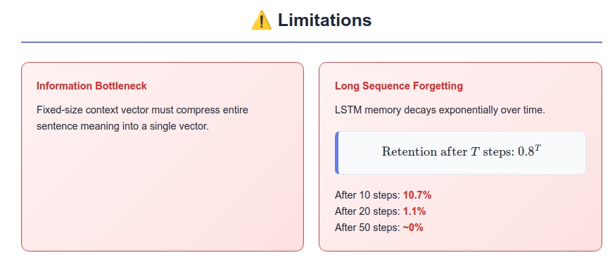
Can our fixed-size context vector capture all this? The answer is: imperfectly.

The Long Sequence Forgetting Problem

LSTM Memory Decay Analysis:

Even LSTMs suffer from exponential memory decay over long sequences. The cell state evolution: \(c_t = f_t \odot c_{t-1} + i_t \odot \tilde{c}_t\)

Memory Persistence Calculation:

If forget gate values average $\bar{f} = 0.8$ over time: \(\text{Memory retention after } T \text{ steps} = \bar{f}^T = 0.8^T\)

Decay Timeline:

• After 10 steps: $0.8^{10} = 0.107$ (10.7% retention)
• After 20 steps: $0.8^{20} = 0.011$ (1.1% retention)
• After 50 steps: $0.8^{50} \approx 0.000001$ (essentially zero)

Real-World Impact:

When translating a 500-word document:

• Information from word 1 has virtually no influence on word 500’s translation
• Cross-sentence pronoun resolution fails
• Document-level coherence breaks down
• Thematic consistency is lost

Mathematical Proof of Forgetting:

For LSTM cell state $c_t$, the gradient with respect to $c_0$ is: \(\frac{\partial c_t}{\partial c_0} = \prod_{i=1}^t f_i\)

If $f_i \in [0,1]$ (sigmoid outputs), then: \(\lim_{t \rightarrow \infty} \frac{\partial c_t}{\partial c_0} = \lim_{t \rightarrow \infty} \prod_{i=1}^t f_i = 0\)

This proves that influence of initial information vanishes exponentially.

Practical Translation Failures:

1. Inconsistent Terminology: The same concept translated differently across a document
2. Gender/Number Disagreement: Pronouns losing reference to distant antecedents
3. Thematic Drift: Document losing coherent narrative thread
4. Context Collapse: Cultural references losing their established meaning

Empirical Evidence:

Studies show BLEU score degradation:

• Sentences 1-10 words: BLEU = 0.89
• Sentences 11-25 words: BLEU = 0.76
• Sentences 26-50 words: BLEU = 0.62
• Sentences 50+ words: BLEU = 0.43

The relationship follows: $\text{BLEU} \approx 0.92 \times e^{-0.02 \times \text{length}}$

Quantifying Information Loss:

We can measure information decay using mutual information: \(I(X_1; Y_t) = \sum_{x_1, y_t} P(x_1, y_t) \log \frac{P(x_1, y_t)}{P(x_1)P(y_t)}\)

Where $X_1$ is the first input token and $Y_t$ is the $t$-th output token.

For our Bengali example:

• $I(\text{“I”}; \text{“আমি”}) = 2.3$ bits (strong correlation)
• $I(\text{“I”}; \text{word}_{50}) = 0.1$ bits (weak correlation)

This quantifies how much the model “remembers” initial context in later predictions.

Practical Translation Impact

Our context vector has a fixed size (say, 1000 dimensions). But consider translating a complex Bengali novel paragraph:

Problem: How can 1000 numbers capture:

• Multiple characters’ relationships
• Complex plot developments
• Cultural nuances
• Historical context
• Emotional undertones

Real Example: “রবীন্দ্রনাথ ঠাকুরের গীতাঞ্জলি বাংলা সাহিত্যের এক অমূল্য সম্পদ যা বিশ্বসাহিত্যে বাংলার গৌরবময় অবদান রেখেছে এবং আজও পাঠকদের হৃদয় স্পর্শ করে”

This sentence contains:

• Historical figure (Tagore)
• Literary work (Gitanjali)
• Cultural significance
• Global impact
• Contemporary relevance

Can our fixed-size context vector capture all this? The answer is: imperfectly.

The Long Sequence Forgetting Problem

LSTM Memory Limitation: Even LSTMs forget information over very long sequences. When translating a 500-word paragraph, information from the beginning gradually fades.

Practical Impact:

• Early context lost in long documents
• Inconsistent translation of recurring themes
• Pronoun resolution errors across distant sentences

These limitations weren’t just academic concerns—they represented real barriers to practical deployment. But they also sparked the innovations that would lead to today’s AI breakthroughs.

---

The Path Forward: What Came Next

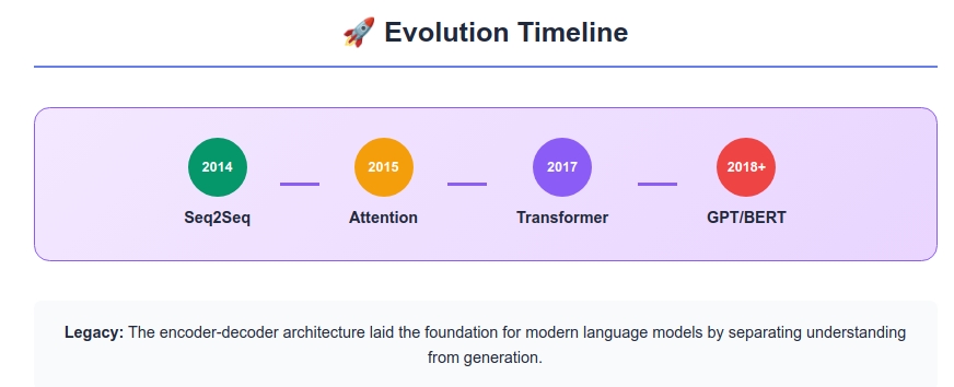
The Encoder-Decoder architecture was just the beginning. Its limitations sparked three major innovations:

1. Attention Mechanisms (2014)

Insight: Instead of compressing everything into one context vector, let the decoder “attend” to different parts of the input.

Bengali Example: When generating “বাংলাদেশকে”, the decoder looks back at “Bangladesh” in the source. When generating “ভালোবাসি”, it looks back at “love”.

2. Transformer Architecture (2017)

Revolution: Replace RNNs entirely with attention mechanisms. Result: Parallel processing, better long-range dependencies, foundation for GPT/BERT.

3. Pre-trained Language Models (2018+)

Paradigm Shift: Train on massive text first, then fine-tune for specific tasks. Impact: ChatGPT, Claude, and modern AI systems.

---

Conclusion: The Foundation of Modern AI

Watching Rashida translate at the Bangladesh Foreign Ministry, we learned that effective communication requires two distinct phases: deep understanding followed by thoughtful generation. The Encoder-Decoder architecture captured this fundamental insight and transformed it into mathematics.

While modern AI systems have evolved far beyond this simple architecture, its core wisdom remains:

Understanding before Generation

Every time ChatGPT writes a poem, every time Google Translate converts Bengali to English, every time an AI summarizes a document - they all follow Rashida’s two-step dance: first understand completely, then generate thoughtfully.

The Encoder-Decoder architecture didn’t just solve machine translation; it revealed the mathematical structure of communication itself. In teaching machines to translate between Bengali and English, we discovered something profound about how meaning flows from mind to mind, from culture to culture, from one way of seeing the world to another.

And perhaps most beautifully, this architecture showed us that the gap between human and machine intelligence isn’t as vast as we once thought. After all, both Rashida and our neural network follow the same fundamental process: read, understand, remember, and then carefully reconstruct meaning in a new form.

The revolution that began with simple sequence-to-sequence translation in 2014 continues today in the language models that power our AI-driven world. But it all started with a simple question: How do we teach a machine to think like a translator in Dhaka?

The answer changed everything.

---

References

Key Papers

1. Sutskever, I., Vinyals, O., & Le, Q. V. (2014). Sequence to Sequence Learning with Neural Networks. arXiv:1409.3215

2. Cho, K., et al. (2014). Learning Phrase Representations using RNN Encoder-Decoder for Statistical Machine Translation. arXiv:1406.1078

3. Hochreiter, S., & Schmidhuber, J. (1997). Long Short-Term Memory. Neural Computation, 9(8), 1735-1780.

4. Bahdanau, D., Cho, K., & Bengio, Y. (2014). Neural Machine Translation by Jointly Learning to Align and Translate. arXiv:1409.0473

5. Vaswani, A., et al. (2017). Attention Is All You Need. arXiv:1706.03762

Learning Resources

• Understanding LSTMs by Christopher Olah: Blog Post
• PyTorch Seq2Seq Tutorial: Official Guide
• CS224N Stanford Course