NumPy - A Beginner's Guide to Numerical Computing in Python

NumPy is a fundamental library for scientific computing in Python. It provides support for large, multi-dimensional arrays and matrices, along with a collection of mathematical functions to operate on these arrays efficiently. In this guide, we’ll explore the basics of NumPy and how it can supercharge your data manipulation and analysis tasks.

Table of Contents

1. Introduction to NumPy
2. Creating NumPy Arrays
3. Array Indexing and Slicing
4. Array Operations
5. Broadcasting
6. Universal Functions (ufuncs)
7. Linear Algebra with NumPy
8. Random Number Generation
9. Conclusion and Further Resources

Introduction to NumPy

NumPy is the foundation for many scientific and data analysis libraries in Python. It provides a powerful N-dimensional array object, tools for integrating C/C++ code, and useful linear algebra, Fourier transform, and random number capabilities.

To get started, you’ll need to install NumPy. You can do this using pip:

pip install numpy

Once installed, you can import NumPy in your Python script:

import numpy as np

Why use NumPy?

NumPy is essential because it provides a fast and memory-efficient way to work with large arrays and matrices. Python lists are great for general-purpose programming, but they become slow and memory-intensive when dealing with large numerical datasets. NumPy’s arrays are stored at one continuous place in memory, allowing for faster access and manipulation.

How to use NumPy?

We import NumPy with the alias np by convention. This allows us to access NumPy functions and classes using the np prefix, making our code more readable and consistent with common practices in the Python scientific community.

Official NumPy Documentation

Creating NumPy Arrays

Let’s start by creating some NumPy arrays:

import numpy as np

# Create a 1D array
arr1d = np.array([1, 2, 3, 4, 5])
print("1D array:", arr1d)

# Create a 2D array
arr2d = np.array([[1, 2, 3], [4, 5, 6]])
print("2D array:\n", arr2d)

# Create an array of zeros
zeros = np.zeros((3, 3))
print("Array of zeros:\n", zeros)

# Create an array of ones
ones = np.ones((2, 4))
print("Array of ones:\n", ones)

# Create an array with a range of values
range_arr = np.arange(0, 10, 2)
print("Range array:", range_arr)

Array Creations 2d Array Why create arrays this way?

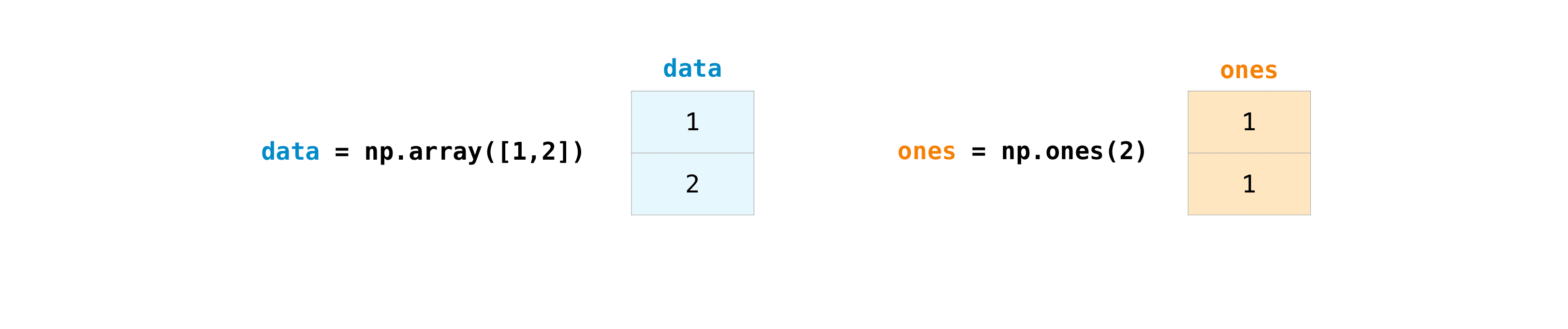
Creating arrays is the first step in working with NumPy. We create arrays to store and manipulate numerical data efficiently. Different array creation methods serve various purposes:

1. np.array(): Creates an array from a Python list or tuple. This is useful when you have existing data you want to convert to a NumPy array.
2. np.zeros() and np.ones(): Create arrays filled with 0s or 1s. These are often used as placeholders or to initialize arrays before filling them with data.
3. np.arange(): Creates an array with a sequence of numbers. This is useful for creating evenly spaced values or as indices.

How does it work?

• np.array() takes a list-like object and creates a NumPy array from it. For 2D arrays, we use nested lists.
• np.zeros() and np.ones() take a tuple specifying the shape of the array (rows, columns).
• np.arange() works similarly to Python’s range() function but returns a NumPy array. It takes start, stop, and step arguments.

NumPy Array Creation Documentation

Array Indexing and Slicing

NumPy arrays can be indexed and sliced similarly to Python lists, but with some powerful extensions:

import numpy as np

arr = np.array([[1, 2, 3, 4], [5, 6, 7, 8], [9, 10, 11, 12]])

# Indexing
print("Element at (1, 2):", arr[1, 2])

# Slicing
print("First two rows, all columns:\n", arr[:2, :])
print("All rows, last two columns:\n", arr[:, -2:])

# Boolean indexing
mask = arr > 5
print("Elements greater than 5:\n", arr[mask])

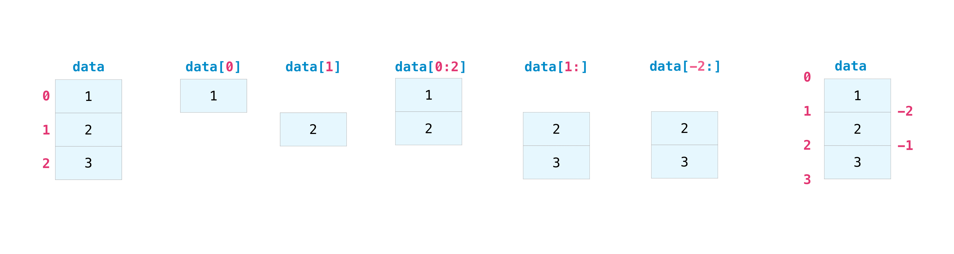1d Slicing 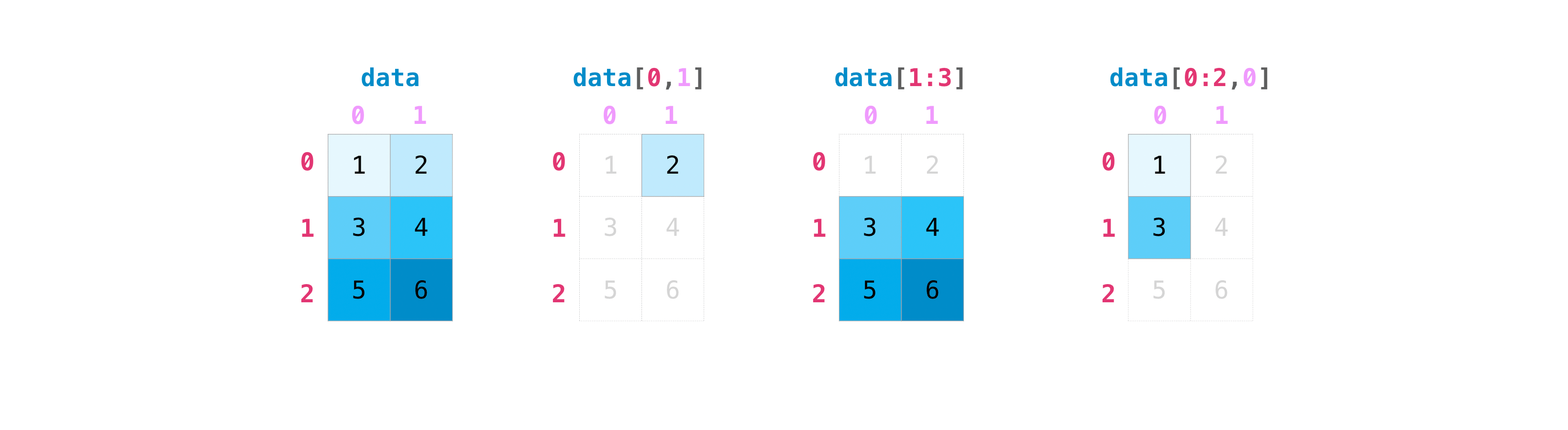Matrix Slicing

Why use array indexing and slicing?

Indexing and slicing allow us to access and manipulate specific elements or subsets of an array. This is crucial for data analysis and manipulation tasks where we often need to work with portions of our data.

How does it work?

• Basic indexing: We use square brackets [] with comma-separated indices for each dimension. For example, arr[1, 2] accesses the element in the second row, third column.
• Slicing: We use the colon : to specify a range. arr[:2, :] selects the first two rows and all columns.
• Negative indexing: Negative indices count from the end. arr[:, -2:] selects all rows and the last two columns.
• Boolean indexing: We create a boolean mask (an array of True/False values) and use it to select elements. arr[arr > 5] selects all elements greater than 5.

NumPy Indexing Documentation

Array Operations

NumPy allows for efficient element-wise operations on arrays:

import numpy as np

a = np.array([1, 2, 3])
b = np.array([4, 5, 6])

# Element-wise addition
print("a + b =", a + b)

# Element-wise multiplication
print("a * b =", a * b)

# Scalar multiplication
print("2 * a =", 2 * a)

# Element-wise exponential
print("a ** 2 =", a ** 2)

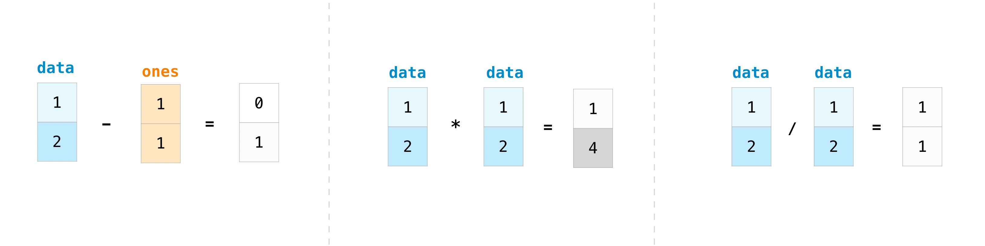
Why use array operations?

Array operations in NumPy are incredibly efficient and allow us to perform calculations on entire arrays without explicit loops. This leads to cleaner, more readable code and significantly faster execution times, especially for large datasets.

How do array operations work?

• Element-wise operations: When you perform operations like +, -, *, / between arrays of the same shape, NumPy applies the operation to each corresponding element pair.
• Scalar operations: When you perform an operation between an array and a scalar (like 2 * a), NumPy applies the operation to every element in the array.
• These operations are vectorized, meaning they’re implemented in compiled C code, making them much faster than equivalent operations using Python loops.

NumPy Operations

Broadcasting

Broadcasting is a powerful mechanism that allows NumPy to work with arrays of different shapes when performing arithmetic operations:

import numpy as np

# Broadcasting example
a = np.array([[1, 2, 3], [4, 5, 6]])
b = np.array([10, 20, 30])

print("a:\n", a)
print("b:", b)
print("a + b:\n", a + b)

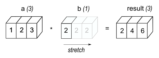
Why use broadcasting?

Broadcasting allows us to perform operations on arrays of different shapes without needing to explicitly expand the smaller array to match the larger one. This saves memory and computation time, and makes the code more concise and readable.

How does broadcasting work?

NumPy compares the shapes of the arrays element-wise, starting from the rightmost dimension. It ‘broadcasts’ the smaller array across the larger array so that they have compatible shapes. Rules for broadcasting are:

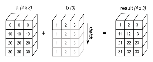
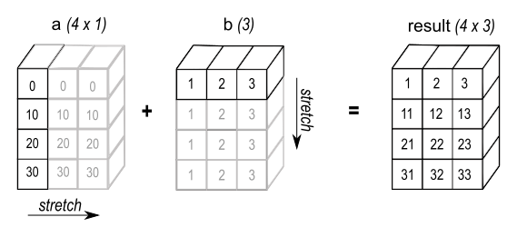
1. If the arrays don’t have the same number of dimensions, the shape of the smaller array is padded with ones on the left.
2. If the shape of the arrays doesn’t match in any dimension, the array with shape equal to 1 in that dimension is stretched to match the other shape.
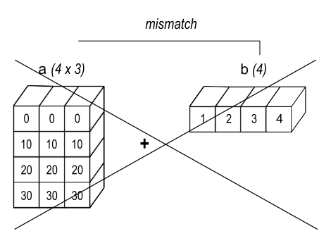
3. If in any dimension the sizes disagree and neither is equal to 1, an error is raised.

In our example, b is broadcasted to match the shape of a, effectively becoming [[10, 20, 30], [10, 20, 30]] for the addition operation.

NumPy Broadcasting Documentation

Universal Functions (ufuncs)

NumPy’s universal functions (ufuncs) operate element-wise on arrays, producing an array as output:

import numpy as np

arr = np.array([-4, -2, 0, 2, 4])

print("Original array:", arr)
print("Absolute values:", np.abs(arr))
print("Exponential:", np.exp(arr))
print("Square root of absolute values:", np.sqrt(np.abs(arr)))

Why use ufuncs?

Universal functions (ufuncs) provide a fast, element-by-element array operation. They are vectorized wrappers of simple functions that take one or more scalar values and produce one or more scalar results. Ufuncs are important because they are much faster than using Python’s built-in functions or loops.

How do ufuncs work?

• Ufuncs operate element-wise on arrays, automatically looping over all elements.
• They can take one input (unary ufuncs) or two inputs (binary ufuncs).
• Ufuncs return a new array with the results, leaving the original array unchanged.
• They support broadcasting, allowing operations between arrays of different shapes.

In our example:

• np.abs() calculates the absolute value of each element.
• np.exp() calculates e raised to the power of each element.
• np.sqrt() calculates the square root of each element. We combine it with np.abs() to avoid errors with negative numbers.

NumPy Universal Functions Documentation

Linear Algebra with NumPy

NumPy provides a comprehensive set of linear algebra operations:

import numpy as np

# Create matrices
A = np.array([[1, 2], [3, 4]])
B = np.array([[5, 6], [7, 8]])

print("Matrix A:\n", A)
print("Matrix B:\n", B)

# Matrix multiplication
C = np.dot(A, B)
print("A dot B:\n", C)

# Compute eigenvalues
eigenvalues = np.linalg.eigvals(A)
print("Eigenvalues of A:", eigenvalues)

# Solve linear equations
x = np.linalg.solve(A, np.array([1, 2]))
print("Solution to Ax = [1, 2]:", x)

Why use NumPy for linear algebra?

NumPy provides efficient implementations of many linear algebra operations. These are essential for various scientific and engineering applications, machine learning algorithms, and data analysis tasks. Using NumPy’s linear algebra functions is much faster and more memory-efficient than implementing these operations manually.

How does NumPy’s linear algebra work?

• Matrix operations: NumPy provides functions like np.dot() for matrix multiplication. It uses optimized, compiled code for these operations, making them very fast.
• Eigenvalues and eigenvectors: np.linalg.eigvals() computes the eigenvalues of a matrix, which are important in many applications, including Principal Component Analysis (PCA) in data science.
• Solving linear equations: np.linalg.solve() solves the linear equation Ax = b for x, where A is a matrix and b is a vector. This is much more efficient than inverting the matrix and then multiplying.

In our example:

• We perform matrix multiplication with np.dot(A, B).
• We compute the eigenvalues of matrix A using np.linalg.eigvals(A).
• We solve the linear equation Ax = [1, 2] using np.linalg.solve(A, np.array([1, 2])).

NumPy Linear Algebra Documentation

Random Number Generation

NumPy’s random module provides a wide variety of probability distributions:

import numpy as np

# Set a seed for reproducibility
np.random.seed(42)

# Generate random integers
random_ints = np.random.randint(1, 11, size=5)
print("Random integers:", random_ints)

# Generate random floats
random_floats = np.random.random(5)
print("Random floats:", random_floats)

# Generate numbers from a normal distribution
normal_dist = np.random.normal(loc=0, scale=1, size=5)
print("Normal distribution:", normal_dist)

Why use NumPy for random number generation?

Random number generation is crucial in many areas of scientific computing, simulations, and data analysis. NumPy’s random module provides a wide range of probability distributions and is designed to be fast and to produce high-quality random numbers.

How does NumPy’s random number generation work?

• Seeding: np.random.seed() sets the starting point for generating random numbers. This is important for reproducibility in scientific experiments and debugging.
• np.random.randint(): Generates random integers from a specified range. It’s useful for simulations, random sampling, and generating random indices.
• np.random.random(): Generates random floats in the half-open interval [0.0, 1.0). This is useful for generating probabilities or random percentages.
• np.random.normal(): Generates random numbers from a normal (Gaussian) distribution. This is widely used in statistics and machine learning for modeling real-world phenomena.

In our example:

• We set a seed for reproducibility.
• We generate 5 random integers between 1 and 10 (inclusive).
• We generate 5 random floats between 0 and 1.
• We generate 5 random numbers from a normal distribution with mean 0 and standard deviation 1.

NumPy Random Sampling Documentation

Conclusion and Further Resources

This guide has only scratched the surface of what NumPy can do. As you continue your journey with NumPy, here are some additional resources to explore:

1. NumPy User Guide
2. NumPy Tutorials
3. SciPy Lectures
4. Python Data Science Handbook

Remember, practice is key to mastering NumPy. Try to incorporate these concepts into your data analysis projects, and don’t hesitate to refer back to the documentation when you need help.

Happy coding with NumPy!

Best of luck

Ahammad Nafiz