Building Neural Networks From Scratch A Step-by-Step Guide

Introduction

Imagine you’re standing at the edge of a vast technological frontier. In one hand, you hold complex mathematical equations that describe how our brains might work. In the other, elegant code that can transform these equations into machines that learn. Welcome to the fascinating world of neural networks.

Neural networks have revolutionized artificial intelligence, powering everything from image recognition to natural language processing. But behind their impressive capabilities lies a surprisingly accessible core of concepts that anyone with basic programming knowledge can understand.

In this comprehensive guide, we’ll journey from the fundamental building blocks of neural networks to implementing a flexible, multi-layer network from scratch using only NumPy. By the end, you’ll not only understand how neural networks work but also have created your own that can tackle real classification problems.

The Story of Neural Networks

Neural networks begin with a simple inspiration: the human brain. Our brains contain billions of neurons, each connected to thousands of others, forming complex networks that enable us to learn, reason, and perceive the world. Artificial neural networks aim to capture this learning capability in mathematical models.

Imagine a child learning to recognize cats. At first, they notice simple patterns – fur, pointy ears, whiskers. Over time, they combine these features to identify a cat, regardless of its color, size, or position. Neural networks learn in a similar way, starting with simple patterns and building up to complex concepts.

The journey of artificial neural networks began in the 1940s with the perceptron, a simple model that could perform basic classification tasks. However, it wasn’t until the 1980s and the introduction of backpropagation that neural networks began to show real promise. The final breakthrough came in the 2010s when increased computing power and data availability catalyzed the deep learning revolution.

Today, we stand on the shoulders of these developments, with the privilege of being able to implement these powerful learning systems in just a few hundred lines of code.

The Neural Network Journey: A Mathematical Adventure

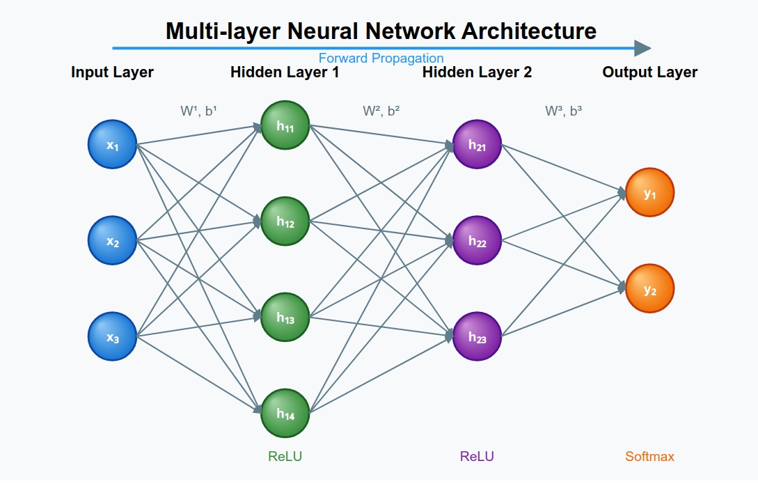
Chapter 1: The Forward Path - How Information Flows

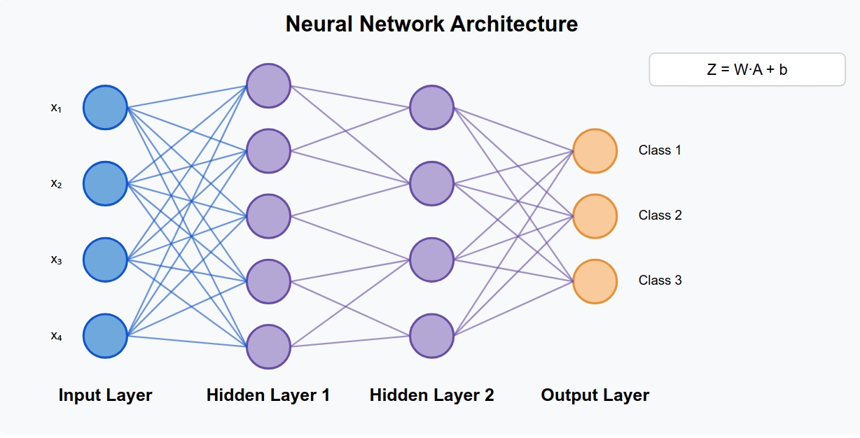
Picture a medieval messenger system between villages. Information travels from the input village (your data) through hidden villages (layers) until it reaches the output village (your prediction). This journey is called forward propagation.

Let’s follow a piece of information as it travels through our network:

Arriving at a Village (Layer \( l \))

When our traveler arrives at village \( l \), it carries information from the previous village. We call this information:

\[A^{[l-1]} \in \mathbb{R}^{n_{l-1} \times m}\]

Think of it this way: \( n_{l-1} \) messengers from the previous village each carry \( m \) different messages – one for each example in our dataset. These messages contain what the previous village learned about our data.

The village has its own system for processing these messages:

• Weights (\( W^{[l]} \)): These determine how important each messenger’s information is
• Biases (\( b^{[l]} \)): These adjust the overall sensitivity of the village to incoming messages

Processing the Information

When a single message arrives, the village processes it like this:

\[Z^{[l](i)} = W^{[l]} A^{[l-1](i)} + b^{[l]}\]

Imagine each messenger’s information being weighed for importance (multiplied by weights), then adjusted by the village’s own biases. This happens for all messages simultaneously:

\[Z^{[l]} = W^{[l]} A^{[l-1]} + b^{[l]}\]

This gives us pre-activation values \( Z^{[l]} \) – the raw, unfiltered information at each village.

Making a Decision

Each village has a special filter (activation function) that determines which information to pass on:

\[A^{[l]} = g^{[l]}(Z^{[l]})\]

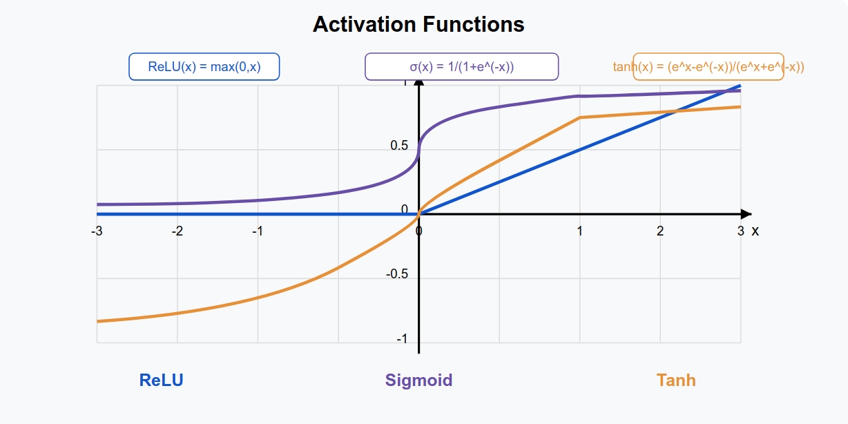
In most villages, they use the ReLU filter – a simple rule that says “pass along any positive information, but ignore anything negative”:

\[\text{ReLU}(z) = \max(0, z)\]

This is like saying: “Only pass along useful, positive signals and filter out the noise.”

The Final Village’s Special Decision Process

The last village uses a special process called softmax to make the final decision:

\[\text{softmax}(z_j) = \frac{e^{z_j}}{\sum_{k=1}^K e^{z_k}} \quad \text{for } j = 1, 2, \ldots, K\]

Think of this as the final village council voting on which category your input belongs to. Each council member (neuron) gets to vote, and the votes are normalized to add up to 1, giving you probabilities for each possible answer.

To make sure no single voice dominates too much, they use a clever trick:

\[\text{softmax}(z_j) = \frac{e^{z_j - \max_k z_k}}{\sum_{k=1}^K e^{z_k - \max_k z_k}}\]

This prevents any one opinion from getting too loud (preventing numerical overflow).

---

Chapter 2: Measuring Success - The Cross-Entropy Tale

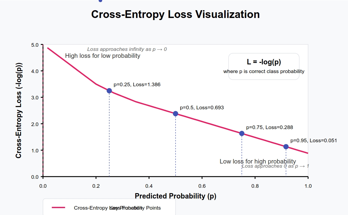
Once the network makes a prediction, we need to know how good it is. Enter cross-entropy loss – our measuring stick for success.

Imagine you’re a weather forecaster predicting rain. You say there’s an 80% chance of rain, but it actually rains 100% (it definitely rains). How wrong were you? Cross-entropy measures this difference:

\[H(p, q) = -\sum_x p(x) \log q(x)\]

Where \( p \) represents the true weather (100% rain) and \( q \) your prediction (80% rain).

For a single training example \( i \):

\[L^{(i)} = -\sum_{j=1}^{K} y_{ij} \log a_{ij}\]

Where \( y_{ij} \) is the true label (1 if the example belongs to class j, 0 otherwise) and \( a_{ij} \) is our prediction probability.

For all our examples together:

\[L = \frac{1}{m} \sum_{i=1}^m L^{(i)} = -\frac{1}{m} \sum_{i=1}^{m} \sum_{j=1}^{K} y_{ij} \log a_{ij}\]

This gives us one number that tells us how wrong our network is across all examples. Lower is better!

---

Chapter 3: The Journey Back - Learning from Mistakes

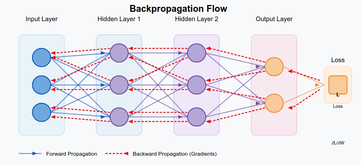
Now comes the magic of neural networks: they learn from their mistakes through backpropagation.

Imagine our network as a complex machine with many knobs (weights and biases). After making a prediction and measuring the error, we need to figure out which knobs to adjust and by how much.

The Goal

We need to calculate:

\[\frac{\partial L}{\partial W^{[l]}}, \quad \frac{\partial L}{\partial b^{[l]}}\]

These tell us how much each weight and bias affects our final error. Think of it as tracing responsibility for the mistake back through the network.

Using the chain rule from calculus:

\[\frac{\partial L}{\partial W^{[l]}} = \frac{\partial L}{\partial Z^{[l]}} \cdot \frac{\partial Z^{[l]}}{\partial W^{[l]}} \quad \Rightarrow \quad dZ^{[l]} = \frac{\partial L}{\partial Z^{[l]}}\]

This is like asking: “How much did the pre-activation values in this layer contribute to our error, and how much did each weight contribute to those values?”

Final Layer

At the final layer, something wonderful happens. When we use softmax with cross-entropy loss, the math simplifies beautifully:

\[dZ^{[L]} = A^{[L]} - Y\]

This has an intuitive meaning: the error is simply the difference between what we predicted \( A^{[L]} \) and the true answers \( Y \). If we predicted 0.8 probability of “cat” but the image was definitely a cat (1.0), our error is 0.8 - 1.0 = -0.2.

Gradients

Once we know the error contribution of this layer, we calculate how much each weight and bias contributed:

\[\frac{\partial L}{\partial W^{[L]}} = \frac{1}{m} dZ^{[L]} A^{[L-1]^T}\] \[\frac{\partial L}{\partial b^{[L]}} = \frac{1}{m} \sum_{i=1}^{m} dZ^{[L](i)}\]

These formulas tell us: “Adjust weights more if they contributed to bigger errors and if they received stronger signals from the previous layer.”

Hidden Layers

For hidden layers, we propagate the error backwards:

\[dA^{[l]} = W^{[l+1]^T} dZ^{[l+1]}\]

This is like passing responsibility back: “Since you contributed this much to the next layer’s values, and those values caused this much error, here’s your share of the blame.”

For the ReLU activation function:

\[dZ^{[l]} = dA^{[l]} \odot g'^{[l]}(Z^{[l]})\]

Where \( g’^{[l]} \) is the derivative of ReLU:

\[g'^{[l]}(Z^{[l]}) = \begin{cases} 1 & \text{if } Z^{[l]} > 0 \\ 0 & \text{otherwise} \end{cases}\]

This means neurons that were “off” (output was 0) get no blame – they didn’t contribute to the error.

We can simplify this to:

\[dZ^{[l]} = dA^{[l]} \odot (Z^{[l]} > 0)\]

Then calculate each layer’s weight and bias gradients:

\[\frac{\partial L}{\partial W^{[l]}} = \frac{1}{m} dZ^{[l]} A^{[l-1]^T}\] \[\frac{\partial L}{\partial b^{[l]}} = \frac{1}{m} \sum_{i=1}^{m} dZ^{[l](i)}\]

---

Chapter 4: Making Improvements - The Gradient Descent Story

Now that we know which direction to turn each knob, we need to actually turn them – this is gradient descent.

The rules are simple:

\[W^{[l]} = W^{[l]} - \alpha \frac{\partial L}{\partial W^{[l]}}\] \[b^{[l]} = b^{[l]} - \alpha \frac{\partial L}{\partial b^{[l]}}\]

Think of yourself walking down a mountain in fog. You can only feel the ground right around you (the gradient) to determine which direction is downhill. You take a step in that direction (adjust weights and biases), then reassess.

The parameter \( \alpha \) is your learning rate – how big of a step you take each time. Too big, and you might overshoot the bottom; too small, and it will take forever to get there.

Implementing a Neural Network from Scratch: Line-by-Line Code Explanation

Now that we understand the theory, let’s implement our neural network class in Python using NumPy, explaining each line of code in detail.

1. Class Initialization

import numpy as np

class NeuralNetwork:
    def __init__(self, input_size, hidden_layers, output_size, learning_rate=0.01):
        self.L = len(hidden_layers)  # Number of hidden layers
        self.parameters = {}
        self.learning_rate = learning_rate

        # Initialize weights and biases
        layer_dims = [input_size] + hidden_layers + [output_size]

        for l in range(1, len(layer_dims)):
            # He initialization for weights
            self.parameters[f"W{l}"] = np.random.randn(layer_dims[l], layer_dims[l-1]) * (2. / layer_dims[l-1])
            # Zero initialization for biases
            self.parameters[f"b{l}"] = np.zeros((layer_dims[l], 1))

Line-by-Line Explanation:

1. import numpy as np - Imports the NumPy library for efficient numerical operations.

2. class NeuralNetwork: - Defines a new class for our neural network.

3. def __init__(self, input_size, hidden_layers, output_size, learning_rate=0.01): - Constructor method that initializes the neural network with specified parameters:
   • input_size: Number of input features
   • hidden_layers: List of sizes for each hidden layer
   • output_size: Number of output classes
   • learning_rate: Step size for gradient descent (default: 0.01)

4. self.L = len(hidden_layers) - Stores the number of hidden layers as an instance variable.

5. self.parameters = {} - Creates an empty dictionary to store all weights and biases.

6. self.learning_rate = learning_rate - Stores the learning rate as an instance variable.

7. layer_dims = [input_size] + hidden_layers + [output_size] - Creates a list containing the dimensions of all layers (input, hidden, and output).

8. for l in range(1, len(layer_dims)): - Loops through each layer (starting from 1, as layer 0 is the input).

9. self.parameters[f"W{l}"] = np.random.randn(layer_dims[l], layer_dims[l-1]) * (2. / layer_dims[l-1]) - Initializes the weights for layer l using He initialization:
   • np.random.randn(...) generates a matrix of random values from a standard normal distribution
   • (2. / layer_dims[l-1]) scales the weights by $\sqrt{\frac{2}{n_{l-1}}}$ (He initialization)
   • Shape: (neurons in current layer, neurons in previous layer)
10. self.parameters[f"b{l}"] = np.zeros((layer_dims[l], 1)) - Initializes the biases for layer l as a column vector of zeros.
    • Shape: (neurons in current layer, 1)

2. Activation Functions

def relu(self, Z):
    return np.maximum(0, Z)

def relu_derivative(self, Z):
    return np.where(Z > 0, 1, 0)

def softmax(self, Z):
    exp_Z = np.exp(Z - np.max(Z, axis=0, keepdims=True))
    return exp_Z / exp_Z.sum(axis=0, keepdims=True)

Line-by-Line Explanation:

1. def relu(self, Z): - Defines the ReLU activation function.
   • Z is the pre-activation matrix from a layer.
2. return np.maximum(0, Z) - Applies the ReLU function element-wise:
   • If an element is positive, keep it as is.
   • If an element is negative, replace it with 0.

3. def relu_derivative(self, Z): - Defines the derivative of the ReLU function.

4. return np.where(Z > 0, 1, 0) - Returns a matrix of the same shape as Z:
   • 1 where Z > 0 (positive elements)
   • 0 elsewhere (negative or zero elements)

5. def softmax(self, Z): - Defines the softmax activation function for the output layer.

6. exp_Z = np.exp(Z - np.max(Z, axis=0, keepdims=True)) - Computes the exponential of each element in Z after subtracting the maximum value in each column:
   • np.max(Z, axis=0, keepdims=True) finds the maximum value for each example (column)
   • Subtracting this maximum improves numerical stability by preventing overflow
7. return exp_Z / exp_Z.sum(axis=0, keepdims=True) - Normalizes the exponentials to sum to 1 along each column (for each example):
   • exp_Z.sum(axis=0, keepdims=True) computes the sum of exponentials for each example
   • Division converts the values to probabilities that sum to 1

3. Forward Propagation

def forward_propagation(self, X):
    cache = {'A0': X}  # Input Layer
    A_prev = X  # Start with the input
    
    # Loop through hidden layers (1 to self.L)
    for l in range(1, self.L + 1):
        W = self.parameters[f'W{l}']
        b = self.parameters[f'b{l}']
        Z = np.dot(W, A_prev) + b
        A = self.relu(Z)
        
        # Store values for backprop
        cache[f'Z{l}'] = Z
        cache[f'A{l}'] = A
        A_prev = A  # pass to next layer

    # Output Layer (L+1; softmax)
    W = self.parameters[f'W{self.L + 1}']
    b = self.parameters[f'b{self.L + 1}']
    Z = np.dot(W, A_prev) + b
    A = self.softmax(Z)

    # Store final layer values
    cache[f'Z{self.L + 1}'] = Z
    cache[f'A{self.L + 1}'] = A

    return cache

Line-by-Line Explanation:

1. def forward_propagation(self, X): - Defines the forward propagation method.
   • X is the input data, shape: (features, examples)

2. cache = {'A0': X} - Creates a dictionary to store all intermediate values, starting with the input.

3. A_prev = X - Initializes A_prev with the input values.

4. for l in range(1, self.L + 1): - Loops through each hidden layer.

5. W = self.parameters[f'W{l}'] - Retrieves the weights for the current layer.

6. b = self.parameters[f'b{l}'] - Retrieves the biases for the current layer.

7. Z = np.dot(W, A_prev) + b - Computes the pre-activation values:
   • np.dot(W, A_prev) performs matrix multiplication
   • + b adds the bias vector (broadcast automatically to all examples)

8. A = self.relu(Z) - Applies the ReLU activation function.

9. cache[f'Z{l}'] = Z - Stores the pre-activation values for backpropagation.

10. cache[f'A{l}'] = A - Stores the activation values for backpropagation.

11. A_prev = A - Updates A_prev for the next layer.

12. W = self.parameters[f'W{self.L + 1}'] - Retrieves the weights for the output layer.

13. b = self.parameters[f'b{self.L + 1}'] - Retrieves the biases for the output layer.

14. Z = np.dot(W, A_prev) + b - Computes the pre-activation values for the output layer.

15. A = self.softmax(Z) - Applies the softmax activation function to get probabilities.

16. cache[f'Z{self.L + 1}'] = Z - Stores the pre-activation values for the output layer.

17. cache[f'A{self.L + 1}'] = A - Stores the activation values for the output layer.

18. return cache - Returns all stored values for backpropagation.

4. Loss Computation

def compute_loss(self, AL, Y):
    m = Y.shape[1]
    # Small epsilon (1e-8) prevents log(0) errors
    return -np.sum(Y * np.log(AL + 1e-8)) / m

Line-by-Line Explanation:

1. def compute_loss(self, AL, Y): - Defines the loss computation method.
   • AL is the activation of the output layer (predictions)
   • Y is the true labels (one-hot encoded)

2. m = Y.shape[1] - Gets the number of examples.

3. return -np.sum(Y * np.log(AL + 1e-8)) / m - Computes the cross-entropy loss:
   • AL + 1e-8 adds a small constant to prevent log(0) errors
   • np.log(AL + 1e-8) calculates the log of each predicted probability
   • Y * np.log(AL + 1e-8) multiplies each log probability by the true label (0 or 1)
   • np.sum(...) sums across all classes and examples
   • -(...) / m negates and normalizes by the number of examples

5. Backward Propagation

def backward_propagation(self, cache, Y):
    grads = {}
    m = Y.shape[1]

    # Output Layer gradient
    dZ = cache[f'A{self.L + 1}'] - Y
    grads[f'dW{self.L + 1}'] = np.dot(dZ, cache[f'A{self.L}'].T) / m
    grads[f'db{self.L + 1}'] = np.sum(dZ, axis=1, keepdims=True) / m
    
    # Hidden Layer gradients
    for l in range(self.L, 0, -1):
        dA_prev = np.dot(self.parameters[f'W{l + 1}'].T, dZ)
        dZ = dA_prev * self.relu_derivative(cache[f'Z{l}'])

        grads[f'dW{l}'] = np.dot(dZ, cache[f'A{l - 1}'].T) / m
        grads[f'db{l}'] = np.sum(dZ, axis=1, keepdims=True) / m

    return grads

Line-by-Line Explanation:

1. def backward_propagation(self, cache, Y): - Defines the backward propagation method.
   • cache is the dictionary of stored values from forward propagation
   • Y is the true labels (one-hot encoded)

2. grads = {} - Creates an empty dictionary to store all gradients.

3. m = Y.shape[1] - Gets the number of examples.

4. dZ = cache[f'A{self.L + 1}'] - Y - Computes the gradient of the output layer:
   • This is a direct result of the derivative of the cross-entropy loss with softmax activation
5. grads[f'dW{self.L + 1}'] = np.dot(dZ, cache[f'A{self.L}'].T) / m - Computes the gradient for the output layer weights:
   • np.dot(dZ, cache[f'A{self.L}'].T) performs matrix multiplication
   • / m normalizes by the number of examples
6. grads[f'db{self.L + 1}'] = np.sum(dZ, axis=1, keepdims=True) / m - Computes the gradient for the output layer biases:
   • np.sum(dZ, axis=1, keepdims=True) sums across all examples
   • / m normalizes by the number of examples

7. for l in range(self.L, 0, -1): - Loops through each hidden layer backwards.

8. dA_prev = np.dot(self.parameters[f'W{l + 1}'].T, dZ) - Computes the gradient of the activations:
   • np.dot(self.parameters[f'W{l + 1}'].T, dZ) propagates the gradient back through the weights
9. dZ = dA_prev * self.relu_derivative(cache[f'Z{l}']) - Computes the gradient of the pre-activations:
   • self.relu_derivative(cache[f'Z{l}']) calculates the derivative of ReLU
   • dA_prev * ... applies the chain rule

10. grads[f'dW{l}'] = np.dot(dZ, cache[f'A{l - 1}'].T) / m - Computes the gradient for the current layer weights.

11. grads[f'db{l}'] = np.sum(dZ, axis=1, keepdims=True) / m - Computes the gradient for the current layer biases.

12. return grads - Returns all computed gradients.

6. Parameter Updates

def update_parameters(self, grads):
    for l in range(1, self.L + 2):
        self.parameters[f'W{l}'] -= self.learning_rate * grads[f'dW{l}']
        self.parameters[f'b{l}'] -= self.learning_rate * grads[f'db{l}']

Line-by-Line Explanation:

1. def update_parameters(self, grads): - Defines the parameter update method.
   • grads is the dictionary of gradients computed in backward propagation

2. for l in range(1, self.L + 2): - Loops through each layer (including the output layer).

3. self.parameters[f'W{l}'] -= self.learning_rate * grads[f'dW{l}'] - Updates the weights:
   • self.learning_rate * grads[f'dW{l}'] scales the gradient by the learning rate
   • -= subtracts the scaled gradient from the current weights
4. self.parameters[f'b{l}'] -= self.learning_rate * grads[f'db{l}'] - Updates the biases:
   • self.learning_rate * grads[f'db{l}'] scales the gradient by the learning rate
   • -= subtracts the scaled gradient from the current biases

7. Training Loop

def train(self, X_train, Y_train, epochs=1000, print_loss=True):
    for epoch in range(epochs):
        # Forward propagation
        cache = self.forward_propagation(X_train)
        AL = cache[f'A{self.L + 1}']

        # Compute loss
        loss = self.compute_loss(AL, Y_train)

        # Backward propagation
        grads = self.backward_propagation(cache, Y_train)

        # Update parameters
        self.update_parameters(grads)

        if print_loss and epoch % 100 == 0:
            print(f'Epoch {epoch} loss: {loss:.4f}')

Line-by-Line Explanation:

1. def train(self, X_train, Y_train, epochs=1000, print_loss=True): - Defines the training method.
   • X_train is the training data
   • Y_train is the training labels
   • epochs is the number of training iterations
   • print_loss determines whether to print loss information

2. for epoch in range(epochs): - Loops through each training epoch.

3. cache = self.forward_propagation(X_train) - Performs forward propagation with the training data.

4. AL = cache[f'A{self.L + 1}'] - Retrieves the output layer activations (predictions).

5. loss = self.compute_loss(AL, Y_train) - Calculates the loss for the current predictions.

6. grads = self.backward_propagation(cache, Y_train) - Performs backward propagation to compute gradients.

7. self.update_parameters(grads) - Updates the parameters based on the computed gradients.

8. if print_loss and epoch % 100 == 0: - Checks if it’s time to print the loss.

9. print(f'Epoch {epoch} loss: {loss:.4f}') - Prints the current epoch and loss.

8. Prediction Function

def predict(self, X):
    cache = self.forward_propagation(X)
    AL = cache[f'A{self.L + 1}']  # Output layer activation (softmax probabilities)
    
    predictions = np.argmax(AL, axis=0)
    return predictions.reshape(1, -1)

Line-by-Line Explanation:

1. def predict(self, X): - Defines the prediction method.
   • X is the input data

2. cache = self.forward_propagation(X) - Performs forward propagation with the input data.

3. AL = cache[f'A{self.L + 1}'] - Retrieves the output layer activations (probabilities).

4. predictions = np.argmax(AL, axis=0) - For each example, finds the index of the class with the highest probability.
   • axis=0 means we’re finding the maximum along each column
5. return predictions.reshape(1, -1) - Reshapes the predictions to a row vector (1, number of examples).

Understanding the Why, What, and How

Why Multi-Layer Architecture?

Neural networks with multiple layers can learn hierarchical representations of data. The first layer might detect simple patterns, while deeper layers combine these patterns to recognize complex features.

In mathematical terms, a multi-layer architecture allows our model to approximate highly non-linear functions. The Universal Approximation Theorem states that a neural network with a single hidden layer of sufficient width can approximate any continuous function to arbitrary precision. However, deeper networks often require fewer total neurons to approximate the same function.

What Makes ReLU Special?

The ReLU activation function, $ReLU(z) = \max(0, z)$, has several advantages:

1. Computational Efficiency: It’s a simple max operation, making it fast to compute.
2. Non-Saturation: Unlike sigmoid or tanh, ReLU doesn’t saturate for positive values, which helps prevent vanishing gradients.
3. Sparse Activation: ReLU naturally leads to sparse activations since it outputs 0 for all negative inputs.

The derivative of ReLU is: $ReLU’(z) = \begin{cases} 1 & \text{if } z > 0 \ 0 & \text{if } z \leq 0 \end{cases}$

This piecewise function is simple to compute and has a clear mathematical interpretation.

How Does Backpropagation Work?

Backpropagation is based on the chain rule from calculus. For a composition of functions $f(g(h(x)))$, the derivative with respect to $x$ is: $\frac{df}{dx} = \frac{df}{dg} \cdot \frac{dg}{dh} \cdot \frac{dh}{dx}$

In our neural network, this allows us to compute how changes in the weights and biases affect the final loss. The key insight is that we can reuse computations as we propagate backwards through the network.

For example, once we’ve computed $\frac{\partial L}{\partial Z^{[l+1]}}$, we can use it to compute $\frac{\partial L}{\partial A^{[l]}}$, which in turn helps us compute $\frac{\partial L}{\partial Z^{[l]}}$, and so on.

This efficient computation is what makes training deep neural networks practical.

Why He Initialization?

The He initialization scales the weights by $\sqrt{\frac{2}{n_{l-1}}}$, where $n_{l-1}$ is the number of neurons in the previous layer. This scaling factor is carefully chosen to maintain the variance of the activations and gradients across layers, which helps prevent the vanishing and exploding gradient problems.

Without proper initialization, deep networks can be extremely difficult to train because:

1. If weights are too small, the signal shrinks as it passes through each layer until it’s too tiny to be useful.
2. If weights are too large, the signal grows exponentially and explodes.

He initialization works particularly well with ReLU activation functions because it accounts for the fact that ReLU sets approximately half of the activations to zero. The factor of 2 in the numerator compensates for this reduction in variance.

Conclusion

You’ve now journeyed through the mathematical foundations of neural networks and implemented one from scratch using NumPy. This fundamental understanding will serve you well as you explore more advanced topics in deep learning.

Remember that while frameworks like TensorFlow and PyTorch make building neural networks much easier, understanding what happens “under the hood” gives you the insight needed to debug models, design custom architectures, and push the boundaries of what’s possible with deep learning.

As you continue your neural network journey, consider exploring:

• Convolutional Neural Networks (CNNs) for image data
• Recurrent Neural Networks (RNNs) for sequential data
• Transformers for natural language processing
• Reinforcement Learning for decision-making problems

Each of these areas builds upon the core concepts we’ve covered, extending them in fascinating directions.

Happy deep learning!